Module 6 · LDA, mistakes, and thresholds

One picture: two overlapping clouds and a dividing line. LDA models each class’s cloud. A boundary decides the label; the cloud area on the wrong side tells us how often it makes mistakes.

Slides → small steps → practice. Browse the original slides at each topic, or click to enlarge. Keep the formula sheet nearby. Module 5 builds the classification and logistic-regression ideas used here.

1. LDA: which class could have produced this input?

Slide 3 of 6

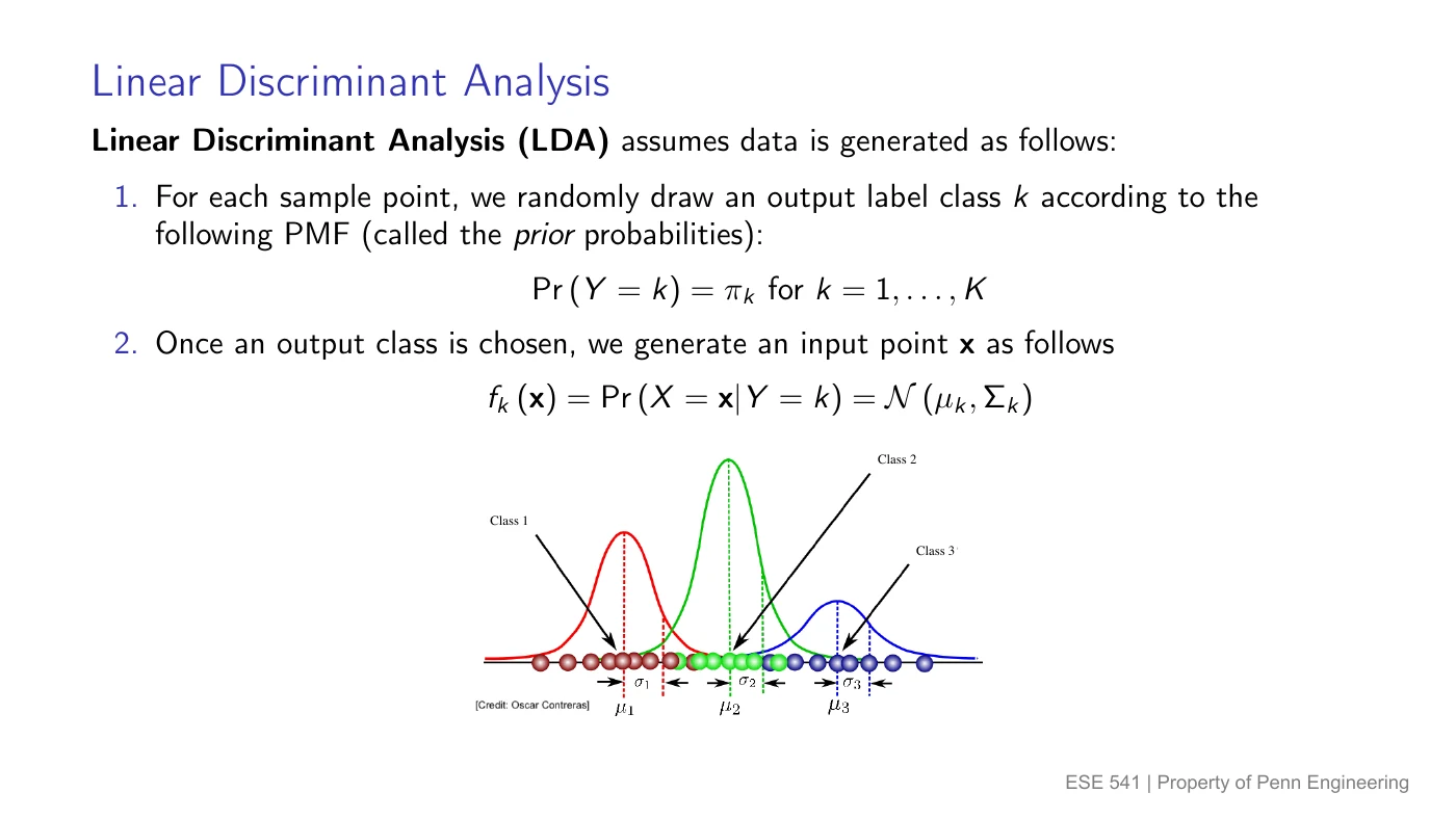
Start with a story for making the data

Linear discriminant analysis (LDA) imagines two steps:

1. Pick a class label $Y=k$. Its prior $\pi_k=P(Y=k)$ is how common that class is before seeing the input.
2. Draw the input $X$ from that class’s bell-shaped, or Gaussian, distribution. Its density is $f_k(x)$.

Here $x$ is the input we observe; $k$ names a class. LDA uses a separate center for each class but a shared spread. With several inputs, it shares the whole covariance matrix: the spread and how inputs vary together.

Density is curve height; probability is area. For a continuous input, $P(X=x)=0$ at one exact point. We use $f_k(x)$ to compare how plausible values near $x$ are within each class. Areas under $f_k$ give probabilities.

Bayes’ rule reverses the story

We observe the input and want the class. The posterior is the updated class probability after seeing $x$:

$K$ is the number of classes; $\ell$ runs through them. The numerator is class frequency × fit to this input. The denominator adds every class’s weight so the answers sum to 1.

Invented example: at one input, suppose priors are $\pi_0=0.8$, $\pi_1=0.2$ and densities are $f_0(x)=0.1$, $f_1(x)=0.3$.

Using total weight $0.08+0.06=0.14$, the posterior for class 1 is $0.06/0.14\approx0.429$. Class 0 wins even though class 1’s density is taller: class 0 started much more common.

The classifier only needs the largest weight

With equal costs for mistakes, choose the most probable class:

$C$ is the classification rule; $\widehat Y$ is its predicted label. Arg max means “return the class label with the biggest value.” The shared denominator cannot change which class wins.

This is Bayes optimal when the probabilities are correct: it minimizes the chance of a wrong label. Fitting LDA from data estimates those probabilities, so its quality depends on both the data and its Gaussian, shared-spread assumptions.

2. One input: turn bell curves into straight scores

Slide 2 of 7

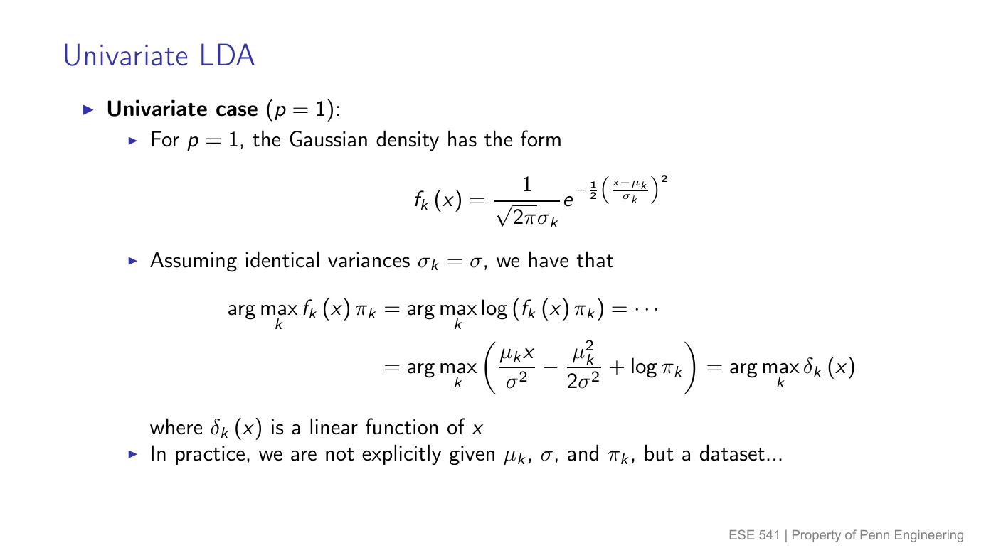
Mean = center; standard deviation = spread

Univariate means one input. Write

The class center is $\mu_k$. The second number, $\sigma^2$, is the variance; its square root $\sigma$ is the standard deviation. LDA uses the same positive variance for all classes.

The Gaussian density is

Here $\pi\approx3.14159$ is the mathematical constant; $\pi_k$ with a subscript is a class prior. Exp means $\exp(a)=e^a$.

Compare a simpler score

Taking logs preserves the ordering of positive weights. After dropping terms shared by all classes, the discriminant score is

$\log$ is the natural logarithm. Choose the class with the largest $\delta_k(x)$. The score is a line in $x$: this is where “linear” comes from. The score itself is not a probability.

Slide example: $\mu_1=-1.5$, $\mu_2=1.5$, shared $\sigma^2=1$, equal priors $0.5$. The squared-mean penalty is the same for both classes: $\mu_k^2/(2\sigma^2)=1.5^2/[2(1)]=1.125$. To find the boundary, set the two scores equal:

Both constants cancel, leaving $-1.5x=1.5x$, so $x=0$. To the right, class 2’s score is larger.

Equal priors put the boundary halfway between the means

For classes 0 and 1 with $\mu_1>\mu_0$, define input boundary $\gamma$:

Predict 1 when $x\geq\gamma$, and 0 otherwise. For equal priors, $\log(1)=0$, so only the midpoint remains. Increasing class 1’s prior moves the boundary left: it takes less input evidence to choose that class.

3. Learn the clouds from data

Usually the centers, spread, and priors are unknown. A hat means estimated from the training data. Let $N$ count all training observations, $K$ count classes, and $N_k$ count observations whose true label is $k$.

Count each class; average within each class

$x_i$ is observation $i$‘s input and $y_i$ is its true label. The sum includes only observations in class $k$.

Pool the leftover spread

Measure each input from its own class mean, square the differences, then combine them:

The denominator is $N-K$ because we estimated $K$ separate means. This is the shared pooled variance. If class sample variances $s_k^2$ are supplied instead:

Invented training data: class 0 has inputs $-2,0$; class 1 has inputs $2,4$. Thus $N=4$, $K=2$, and each $N_k=2$.

• Priors: use $N_k/N$: both are $2/4=0.5$.
• Centers: use each group’s mean: $\widehat\mu_0=(-2+0)/2=-1$ and $\widehat\mu_1=(2+4)/2=3$.
• Spread: each class’s deviations from its own mean are $-1,+1$. Their squared sum is $1+1+1+1=4$; hence $\widehat\sigma^2=4/(4-2)=2$.
• Boundary: equal priors give midpoint $\widehat\gamma=(-1+3)/2=1$.

Several inputs: the same comparison in more directions

Multivariate means several inputs. The input $\mathbf x$ and class center $\boldsymbol\mu_k$ are lists of $p$ numbers, called vectors. A shared $p\times p$ covariance matrix $\Sigma$ records each input’s variance and which inputs tend to move together.

The clouds become ellipses in two dimensions. LDA still compares prior × density. Its boundaries become straight lines in two dimensions and flat separating surfaces in more dimensions.

For the multivariate Gaussian, write the adjusted squared distance as

Then its density is

$\mathbf u_k$ is the offset from the class center. $T$ turns a column into a row; $\Sigma^{-1}$ adjusts distance for spread and correlation; $|\Sigma|$ is the determinant, which scales the cloud’s volume. Use a nonsingular shared covariance matrix. With $p=1$, $d_k^2=(x-\mu_k)^2/\sigma^2$, recovering the one-input formula.

4. Name a mistake before calculating its rate

Slide 2 of 5

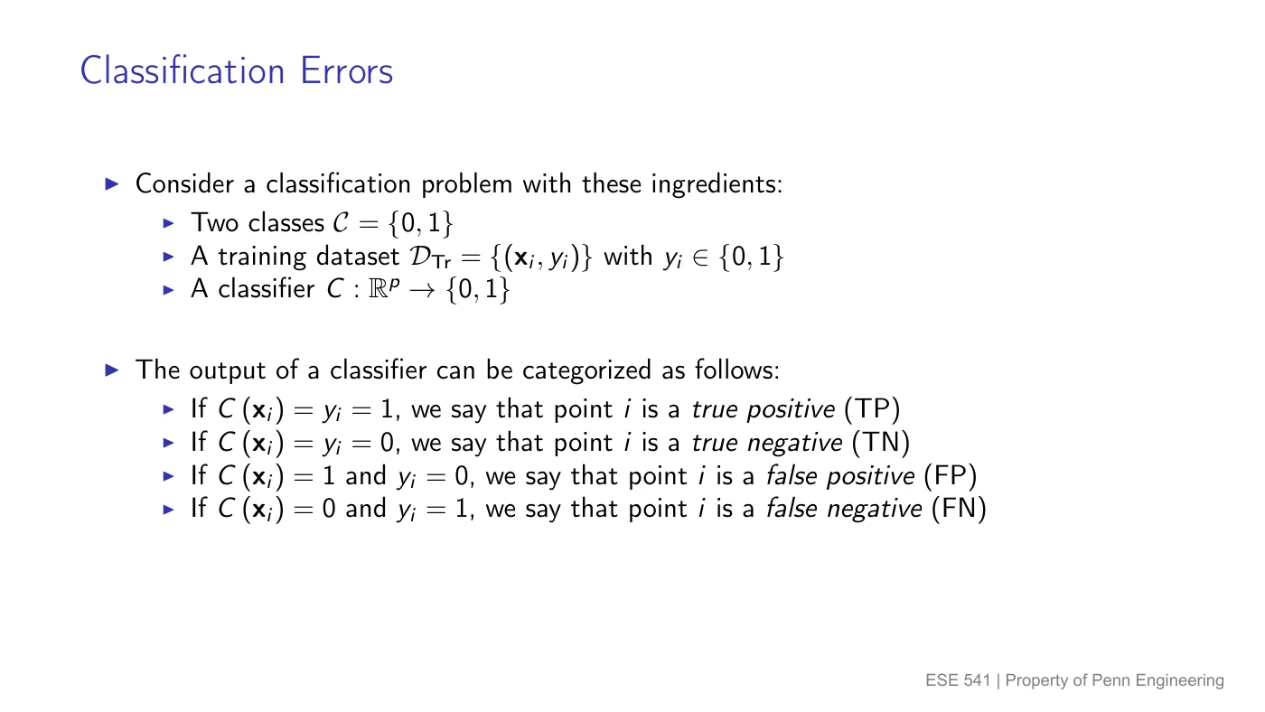
Let positive = class 1, negative = class 0. “Positive” says what the model predicted; “true” or “false” says whether that prediction was correct.

Here TP, FP, TN, and FN stand for counts. With $N$ evaluated observations:

Invented counts: 4 false alarms and 6 missed positives among 100 observations give $(4+6)/100=0.10=10\%$ error.

5. Confusion matrix: always ask “out of which group?”

Slide 3 of 5

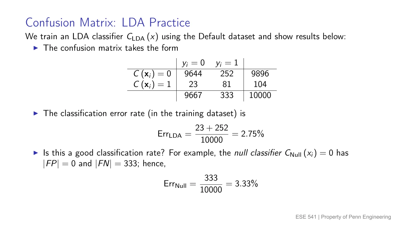
A confusion matrix sorts the four counts into a table. The slides put predictions in rows, actual labels in columns. Other tables may swap them: read the labels first.

The supplied Default example evaluates the fitted classifier on its training data and calls default class 1:

Use the actual class as the denominator

FPR and TNR divide the actual negatives. FNR and TPR divide the actual positives. Each pair adds to 1:

For the slide’s counts:

• False positive rate: $23/(23+9644)=23/9667\approx0.00238=0.238\%$.
• False negative rate: $252/(252+81)=252/333\approx0.7568=75.68\%$.
• True positive rate: $81/(81+252)=81/333\approx0.2432=24.32\%$.
• Overall training error: $(23+252)/10000=0.0275=2.75\%$.

The small overall training error hides a large miss rate for actual defaults. Most observations are class 0. Even the null classifier, which always predicts 0, makes only $333/10000=3.33\%$ errors on these observations, while missing every default. New-data performance requires a separate test set.

FPR is not “out of everything predicted positive.” Its denominator is everything actually negative. Say that group aloud before dividing.

6. Gaussian errors are areas across the boundary

Slide 3 of 4

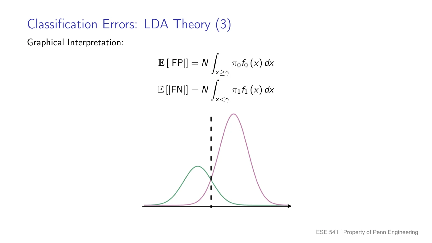
Shade the wrong side of each class’s curve

Suppose we predict 1 for $x\geq\gamma$ and 0 for $x<\gamma$. Each class density has total area 1:

The integral sign means “add up the area.” The first expression shades class 0’s right tail; the second shades class 1’s left tail.

Standardize: how many standard deviations away?

For a normal class with mean $\mu$ and standard deviation $\sigma$:

Let $\Phi(z)$ be the area to the left of $z$ under a standard normal curve, whose mean is 0 and standard deviation is 1. With class means $\mu_0,\mu_1$ and shared $\sigma$:

Then $TPR=1-FNR$.

Invented one-class calculation: if $\mu_0=-2$, $\sigma=1$, and $\gamma=0$, the boundary is $z=[0-(-2)]/1=2$ standard deviations above the center. Its right-tail error is $1-\Phi(2)\approx0.02275$.

Whole-population errors need the priors too

Conditional rates answer “among this actual class.” To find a fraction of everyone, multiply by that class’s prior:

For $N$ observations drawn from that population, expected counts are

$E$ means the long-run average over repeated samples. Invented example: $N=1000$, $\pi_0=0.9$, $\pi_1=0.1$, $FPR=0.02$, and $FNR=0.20$. Expected FP is $1000(0.9)(0.02)=18$; expected FN is $1000(0.1)(0.20)=20$. Total error is $(18+20)/1000=0.038=3.8\%$.

Adding $FPR+FNR=0.22$ would mix rates with different denominators. Weighting them gives the fraction of all observations that are wrong.

7. Move the threshold; trade false alarms for misses

Slide 2 of 5

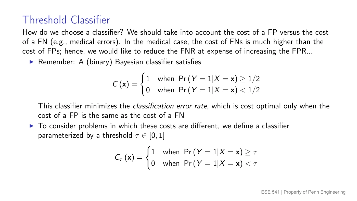
Probability threshold and input boundary are different numbers

Let $p_1(x)=P(Y=1\mid X=x)$ be the posterior for class 1. The probability threshold $\tau$ says how sure we must be before predicting 1:

Equal mistake costs give the usual $\tau=0.5$. A lower $\tau$ predicts 1 more often: it catches more actual positives (TPR rises, FNR falls) while also flagging more actual negatives (FPR rises). Raising $\tau$ reverses that tradeoff. On finite data, rates can stay unchanged between score values.

For the one-input LDA model with $\mu_1>\mu_0$, the corresponding input boundary is

This formula uses $0<\tau<1$. $\tau$ is a probability; $\gamma_\tau$ is measured in the input’s units. If missing a positive costs more, choose a lower probability threshold to put more emphasis on catching positives.

ROC: show every threshold on one graph

The receiver operating characteristic (ROC) curve plots FPR horizontally and TPR vertically as the threshold changes. Every point is a different tradeoff for the same scoring model.

• Near $(0,0)$: predict almost nobody positive.
• Near $(1,1)$: predict almost everybody positive.
• Toward $(0,1)$: catch positives with few false alarms.

AUC means the area under that ROC curve. Higher AUC summarizes better separation across thresholds; it does not choose the operating threshold or the preferred balance of mistakes. A diagonal curve has AUC $0.5$; perfect separation has AUC $1$.

Try the boundary on the actual practice distributions

Use the Q3 and Q7 presets below. Move the boundary right and watch both TPR and FPR fall. Change a prior and notice why the overall error uses a weighted sum even though the conditional curves still each have area 1.

8. Shared practice Q3: two Gaussians centered at −3 and +3

View the original practice sheet (includes solutions)

Page 2 of 6

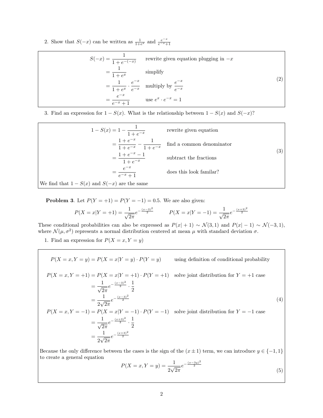
Given: labels $y\in\{-1,+1\}$, both priors $0.5$, and

The shared variance is 1, so the standard deviation is $\sqrt1=1$. Rules: Bayes and joint densities, LDA boundary, and Gaussian tail errors.

1. Joint density = class density × class prior

Write $g(x,y)$ for the joint density in continuous input $x$ and discrete label $y$. The rule is $g(x,y)=f_y(x)P(Y=y)$.

Using means $3y$, variance 1, and prior $1/2$:

For $y=+1$, the squared term is $(x-3)^2$; for $y=-1$, it is $(x+3)^2$. Each joint curve has area $1/2$, because each label occurs half the time. Their two areas add to 1.

2. Draw equal-width curves; split at the midpoint

The conditional densities $f_{-1}(x)$ and $f_{+1}(x)$ have centers $-3,+3$ and each has area 1. Equal priors and equal variance give boundary

At $x=0$ the two posteriors tie, so either label is valid. A single point has zero probability here. The widget’s Q3 preset draws both curves and the boundary.

3. Find the negative class’s right-tail area

Standardize using boundary $0$, negative-class mean $-3$, and standard deviation $1$:

The 99.7% empirical rule puts approximately 0.997 of a normal curve within three standard deviations. The remaining mass splits equally between the two tails:

This is the practice approximation: 0.15% of actual negatives cross the boundary. An exact normal calculation gives $1-\Phi(3)\approx0.001350$, or $0.135\%$. The difference is the empirical rule’s rounding.

The answer is a conditional tail area. Multiplying by the negative prior $0.5$ would instead give the fraction of the entire population that is a false positive.

9. Shared practice Q4: spam is the positive class

Given: a spam detector. Define $Y=1$ as actually spam and $C(x)=1$ as marked spam. Rule: confusion matrix rates.

Memory aid: “false” means wrong; “positive” means the predicted spam label. FPR is a false alarm among legitimate emails. FNR is a miss among spam emails. TPR and FNR divide the same actual-spam group, so $TPR=1-FNR$.

10. Shared practice Q7: decode a noisy 0 or 1

View Q7 on the original practice sheet (includes solutions)

Page 5 of 6

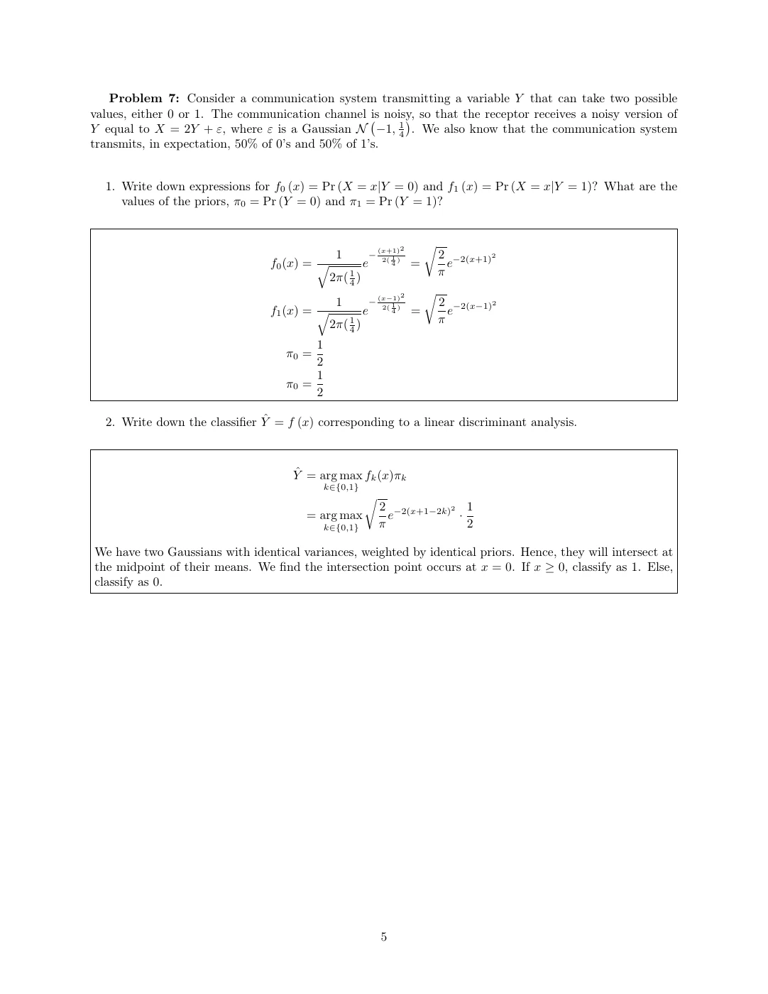
Given: the transmitted bit is $Y\in\{0,1\}$, each bit occurs half the time, and the received input is

Treat the channel noise as having this same distribution for either transmitted bit. Its mean is $-1$ and its variance is $1/4$, so its standard deviation is $\sqrt{1/4}=1/2$.

Rules: shifted Gaussian inputs, LDA boundary, Gaussian tails, and weighted error.

1. Substitute each possible bit

Adding a constant moves a distribution’s mean without changing its variance.

• If $Y=0$, then $X=0+\varepsilon$: mean $2(0)-1=-1$, variance $1/4$.
• If $Y=1$, then $X=2+\varepsilon$: mean $2(1)-1=1$, variance $1/4$.

Thus

The supplied 50/50 transmission frequencies give both priors:

For $k\in\{0,1\}$, the mean is $\mu_k=2k-1$. Substitute this mean and $\sigma^2=1/4$ into the normal density. The front factor becomes $1/[(1/2)\sqrt{2\pi}]=\sqrt{2/\pi}$; the exponent’s multiplier becomes $1/[2(1/4)]=2$. Thus

In particular,

These are densities; their areas, rather than individual heights, give probabilities.

2. Use the midpoint because priors and variances match

The LDA rule chooses the larger $\pi_kf_k(x)$. With equal priors $1/2$, equal variance $1/4$, and means $-1,+1$, the boundary is

3. Compute FPR, then use symmetry for TPR

FPR is among actual zeros. The mean is $-1$, standard deviation $1/2$, and boundary $0$:

Using the practice approximation that 95.4% lies within two standard deviations, the right tail is

FNR is among actual ones. This class has mean $1$, standard deviation $1/2$, and boundary $0$:

The equal-width mirrored curve has left-tail mass $FNR\approx0.023$. Therefore

So approximately 2.3% of actual zeros trigger a false 1, while 97.7% of actual ones are correctly received as 1. Exact normal values are $FPR=FNR\approx0.022750$ and $TPR\approx0.977250$.

4. Weight the two kinds of error by how often each bit occurs

Use the total-error rule, the supplied priors $\pi_0=\pi_1=0.5$, and calculated rates $FPR\approx FNR\approx0.023$:

Invented batch-size illustration: for 1000 transmitted bits, expect 500 actual zeros and 500 actual ones. Expected false positives are $500(0.023)=11.5$ and expected false negatives are also 11.5. Thus approximately 23 of the 1000 bits are wrong. Expected counts can be fractional; any one real batch has whole-number counts.

The exact Gaussian total error is about $0.022750$. The practice’s $0.023$ uses its two-standard-deviation approximation consistently.

11. Pick the calculation that matches the question

The shared sheet’s Q1, Q2, Q5, and Q6 are in Module 5. Reuse the Module 6 formula sheet when the numbers change.