Module 5 · Classification and logistic regression

Classification means choosing a label. First estimate how likely each label is; then choose one. Logistic regression builds those probabilities from the same weighted sums used in regression.

Slides → small steps → practice. Browse the original slides above each topic, or click to enlarge. Keep the formula sheet nearby. This module covers shared practice Q1, Q2, Q5, and Q6; Module 6 covers Q3, Q4, and Q7.

1. A label and a probability are different things

Slide 3 of 4

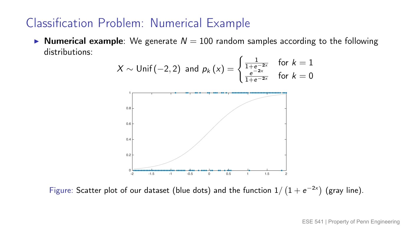
Same inputs can lead to different labels

An email is spam or not spam; it cannot be 0.7 spam. But a model can give it a 70% chance of being spam.

• $X$ is the input, such as email features; $x$ is one particular input.
• $Y$ is the actual label. In a binary problem there are two labels, often 0 and 1.
• $p_k(x)=P(Y=k\mid X=x)$ is the probability of label $k$, given input $x$. The vertical bar means “given.”
• $C(x)$ is a classifier: the rule that chooses a label from the probabilities.

For two classes, the probabilities must add to 1:

Read the slide’s data-generating example

The slide generates 100 examples by first drawing an input uniformly between $-2$ and $2$, then drawing its label:

Uniform means equal-length input intervals are equally likely. $e\approx2.718$ is the exponential base. At input $x=0$, the class-1 chance is $1/(1+e^0)=1/2$. At $x=1$, it is $1/(1+e^{-2})\approx0.881$.

The observed label is still 0 or 1. The smooth curve describes the chance of getting 1 at each input, not a halfway label.

2. Bayes: pick the most likely label

Slide 2 of 5

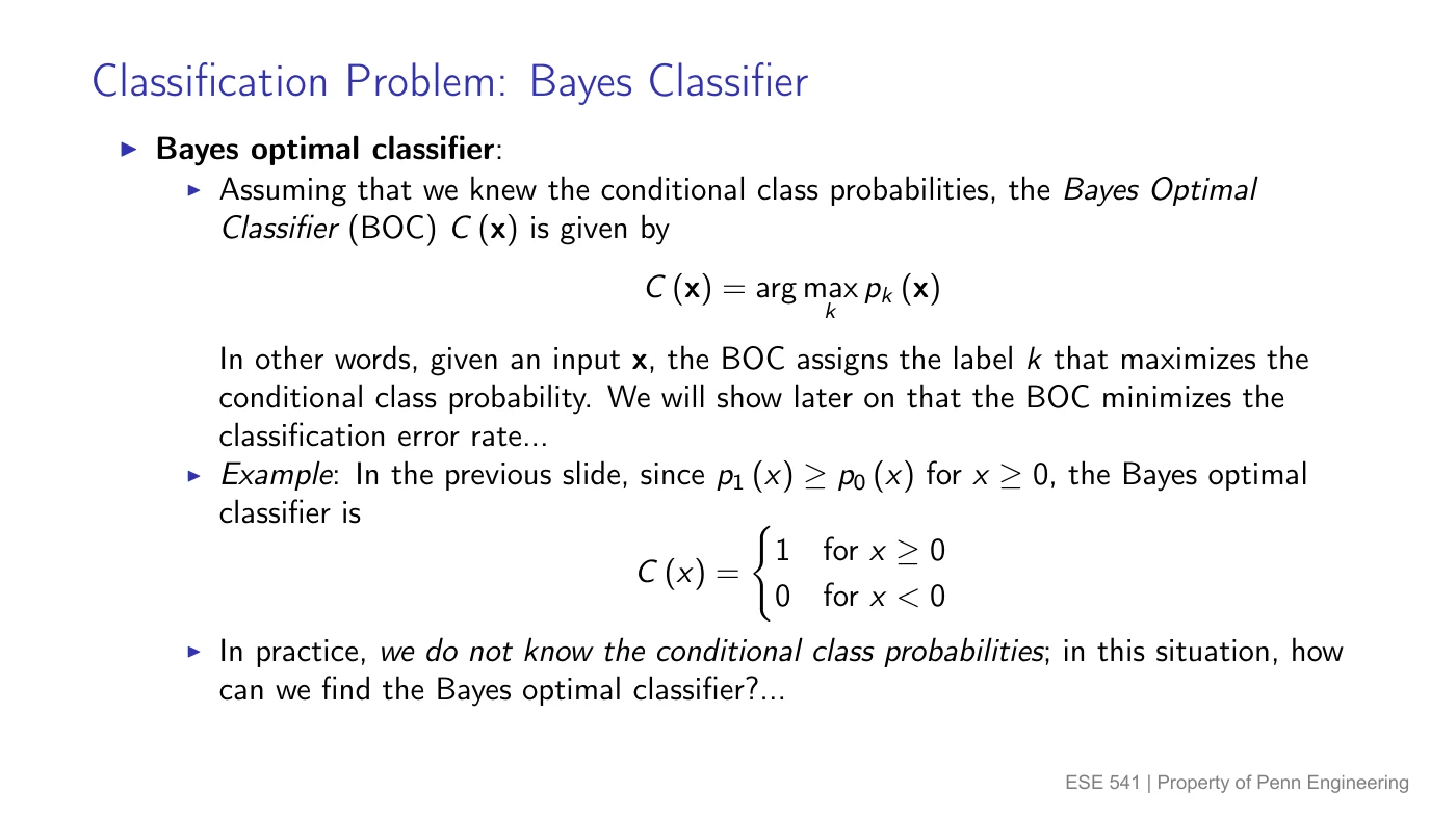
“Optimal” means the smallest possible error rate

If a label has probability 0.8, choosing it gives a 0.2 chance of being wrong. Choosing the other label gives a 0.8 chance of being wrong. Pick the biggest probability to minimize mistakes, when all mistakes count equally.

For $K$ classes, the Bayes classifier is

$K$ counts labels. Arg max means “the label that gives the largest value.” The star marks the ideal rule using the true probabilities.

For labels 0 and 1, choose 1 when $p_1(x)\geq0.5$, and 0 otherwise. At exactly 0.5, either label has the same error; we choose 1 to settle the tie. In the slide’s example, this gives class 1 for $x\geq0$ and class 0 for $x<0$.

Unknown probabilities: estimate from nearby examples

Local averaging asks “among training inputs near this one, what fraction have label 1?” If $\mathcal N(x)$ is a chosen neighborhood containing $m$ observations:

$y_i$ is the observed 0-or-1 label. Adding these labels counts the ones; a hat marks an estimate from data.

Invented neighborhood: labels $1,1,0,1,0$ give $\widehat p_1(x)=3/5=0.6$. Since $0.6\geq0.5$, predict 1.

Curse of dimensionality: with many input features, examples spread out in many directions. A tiny neighborhood may contain almost nobody; a big one includes less similar inputs. Logistic regression addresses this by assuming a specific shape for the probability rule.

3. Logistic regression: score → probability → label

Slide 2 of 3

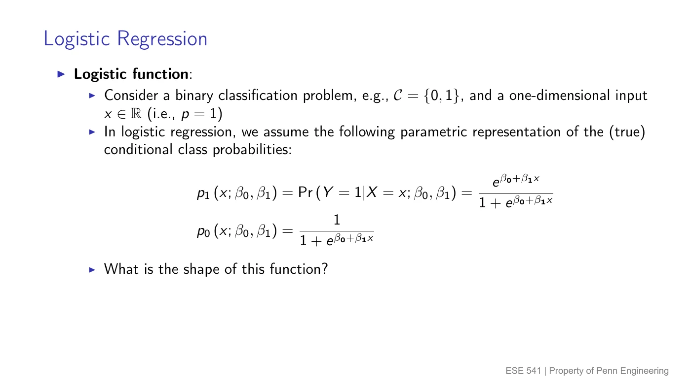
First add contributions

For $d$ input features, make a score $z$:

$\beta_0$ is the intercept; $\beta_j$ multiplies feature $x_j$. We use $d$ for the number of features so it cannot be confused with a probability $p$. The score can be any real number, so it is not yet a probability.

Then squash the score between 0 and 1

The sigmoid, or logistic function, is an S-shaped converter:

Logistic regression assumes

The threshold is the minimum probability needed to predict 1. With threshold 0.5, it is enough to check whether $z\geq0$. The decision boundary is where $z=0$: the prediction switches labels there. Changing the threshold changes decisions without changing fitted probabilities.

What the coefficient actually changes

The odds of class 1 are its probability divided by the probability of class 0. For probability $p=p_1(x)$:

$\ln$ is the natural logarithm, which undoes the exponential. At $p=0.8$, odds are $0.8/0.2=4$: 4 to 1, not 4%.

Holding other inputs fixed, one extra unit of feature $x_j$ adds $\beta_j$ to the log-odds and multiplies the odds by $e^{\beta_j}$. It does not add $\beta_j$ to the probability. A positive coefficient raises the class-1 probability; a negative one lowers it.

4. Maximum likelihood: reward probabilities assigned to actual labels

Slide 2 of 5

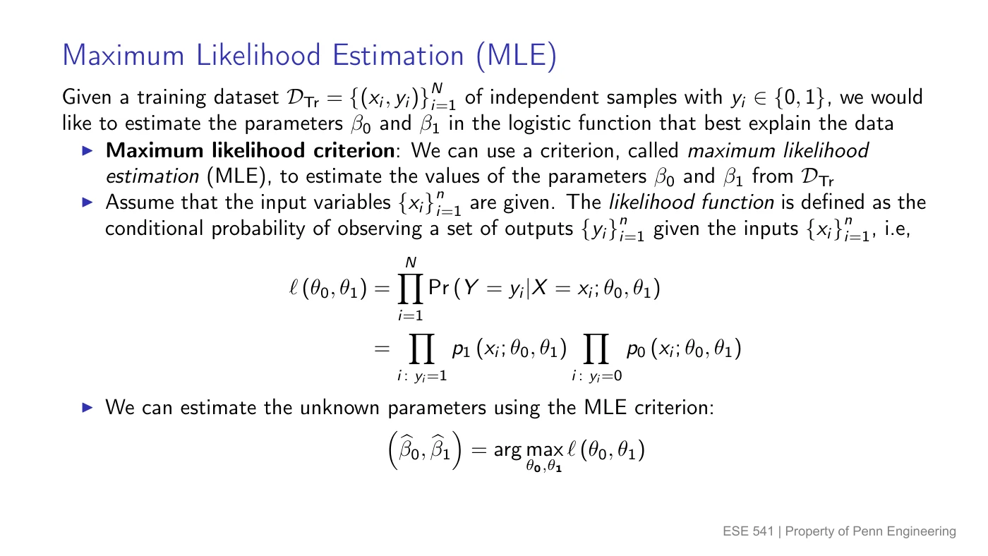
For each row, use the chance of what actually happened

Suppose a candidate model gives row $i$ class-1 probability $p_i=S(\beta_0+\sum_j\beta_jx_{ij})$. Here $x_{ij}$ is feature $j$ of row $i$.

• If the actual label is $y_i=1$, use $p_i$.
• If the actual label is $y_i=0$, use $1-p_i$.

For $n$ independent training examples, multiply these chances to get the likelihood:

$\prod$ means multiply; $\boldsymbol\beta$ means all the coefficients together. The exponents select the correct chance: an exponent of 0 turns the unused factor into 1.

Maximum likelihood estimation (MLE) chooses coefficients that make this product as large as possible:

Invented three-row comparison: actual labels are $1,0,1$.

Candidate A proposes class-1 probabilities $0.8,0.3,0.6$. The likelihood is $0.8(1-0.3)(0.6)=0.336$.

Candidate B proposes class-1 probabilities $0.6,0.4,0.5$. The likelihood is $0.6(1-0.4)(0.5)=0.180$.

Candidate A assigns more probability to the observed combination of labels. Fitting searches for the best coefficients, not just the better of these two candidates. The likelihood scores the observed labels for chosen coefficients; it is not the probability that those coefficients are true.

After fitting, substitute into the score

The slide’s fitted default model uses balance $B$ in dollars:

• At the supplied $B=1000$: $z=-10.65+0.0055(1000)=-5.15$. Thus $\widehat p_1=1/(1+e^{5.15})\approx0.00577$, about 0.6%.
• At the supplied $B=2000$: $z=-10.65+0.0055(2000)=0.35$. Thus $\widehat p_1=1/(1+e^{-0.35})\approx0.5866$, about 58.7% using these rounded coefficients.

5. Hypothesis tests: is a fitted weight clearly different from zero?

Slide 2 of 4

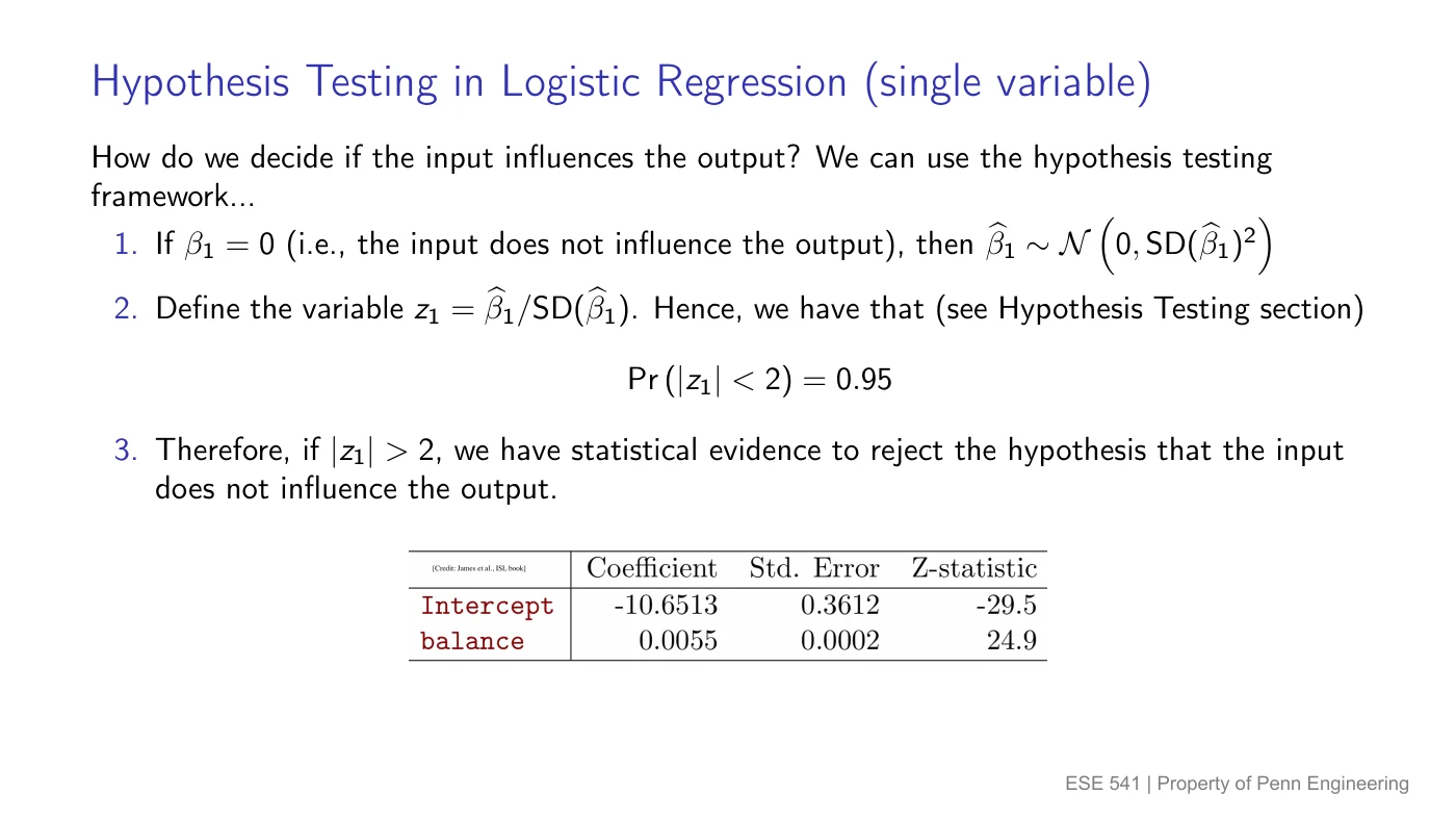
Estimate ÷ uncertainty

The null hypothesis $H_0:\beta_j=0$ says feature $j$ contributes nothing to this model’s score, with other inputs held fixed. The alternative is $\beta_j\neq0$.

The fitted coefficient $\widehat\beta_j$ changes across samples. Its standard error, $\operatorname{SE}(\widehat\beta_j)$, estimates the size of that variation. Measure the distance from zero in standard errors:

This z-statistic is different from the prediction score $z$ above. Under the null and suitable large-sample conditions, it is approximately standard normal. About 95% of that distribution lies between $-2$ and $2$.

Use the module’s approximate rule: reject $H_0$ when $|z_j|>2$; otherwise fail to reject. At exactly 2, this stated rule does not reject.

Invented fit: $\widehat\beta_1=0.6$ and $\operatorname{SE}=0.2$ give $z_1=0.6/0.2=3$. Since $|3|>2$, reject a zero coefficient. This is evidence of association in the model; it does not establish causation. Failing to reject does not prove the coefficient is zero.

With multiple features, add all their contributions to the score, fit all coefficients by MLE, and test each coefficient relative to its own standard error.

6. More than two labels: give each a share of the total

Slide 2 of 3

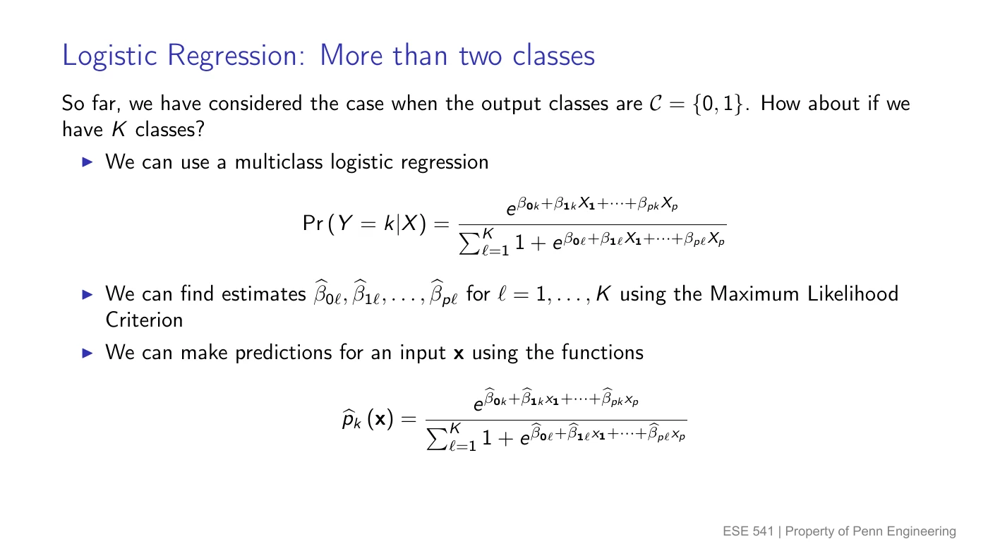
For $K$ classes and $d$ features, give each class $k$ its own weighted score:

$\beta_{0k}$ is class $k$‘s intercept; $\beta_{jk}$ weights feature $j$ for that class. Turn the scores into positive weights $e^{z_k}$, then divide each weight by the total:

This is softmax. The index $\ell$ runs through every class in the denominator, so the probabilities sum to 1. There is no extra 1 when all $K$ classes are already in the sum. If a reference class has score 0, its weight is $e^0=1$; writing that term separately gives $1+$ the sum over the remaining classes.

Invented scores: $z_1=0$, $z_2=\ln2$, $z_3=\ln3$. Exponentiating gives weights $1,2,3$ and total $1+2+3=6$:

Choose class 3, the largest probability. MLE fits the coefficients by maximizing the product of the probabilities assigned to the actual training labels.

7. Shared practice Q1: moving the rectangle

View the original practice sheet (includes solutions)

Slide 1 of 6

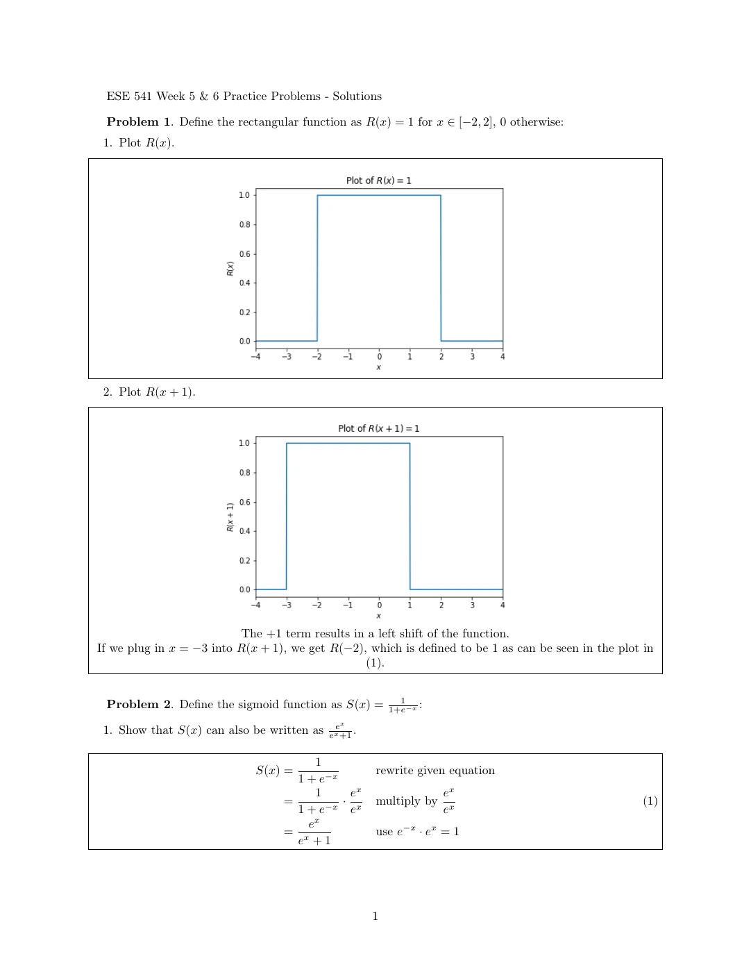
Given: $R(x)=1$ on the inclusive interval $[-2,2]$, and 0 otherwise. Plot $R(x)$ and $R(x+1)$. Rule: horizontal shifts.

Ask which input reaches the “on” interval

$R$ outputs 1 when the number inside its parentheses is between $-2$ and $2$.

For $R(x)$, this is simply $-2\leq x\leq2$. For $R(x+1)$, substitute the inside expression and subtract 1 throughout:

So $R(x+1)$ moves the rectangle left by 1. The height stays 1.

Check the new left endpoint: at $x=-3$, the inside is $-3+1=-2$, so $R(-3+1)=R(-2)=1$. At $x=2$, the inside is 3, so $R(2+1)=0$.

Reusable rule: $f(x+a)$ shifts the graph left by $a$ when $a>0$; $f(x-a)$ shifts it right by $a$.

8. Shared practice Q2: three sigmoid identities

Given: $S(x)=1/(1+e^{-x})$. Rewrite it, evaluate $S(-x)$, and relate $S(-x)$ to $1-S(x)$. Rule: sigmoid identities.

1. Remove the negative exponent

Multiply numerator and denominator by $e^x$. This multiplies the fraction by 1, and $e^xe^{-x}=e^0=1$:

2. Replace every x with −x

Two minus signs cancel in the exponent. Then multiply numerator and denominator by $e^{-x}$ for the second form:

3. Subtract using a common denominator

Write $1=(1+e^{-x})/(1+e^{-x})$, then subtract:

Meaning: reversing the score swaps the two class probabilities. For a numerical check at $x=2$, $S(2)\approx0.8808$ and $S(-2)\approx0.1192$; they add to 1.

9. Shared practice Q5: hours, GPA, and getting an A

Given: 100 students; $X_1$ is hours studied, $X_2$ is GPA, and $Y=1$ means receiving an A. The fitted coefficients are $\widehat\beta_0=-6$, $\widehat\beta_1=0.05$, and $\widehat\beta_2=1$.

Rules: logistic prediction and solving for a target probability.

1. Find the chance at 40 hours and GPA 3.5

Rule: add weighted inputs. With supplied hours $X_1=40$ and GPA $X_2=3.5$:

Rule: put the score into the sigmoid. Using the calculated $z=-0.5$:

The 100 students were used for fitting; you do not divide this prediction by 100.

2. Find hours for a 50% chance, with GPA still 3.5

Rule: a 50% probability means score 0, since $\ln(0.5/(1-0.5))=\ln1=0$. Let $h$ be the required hours. Keep the supplied GPA at 3.5:

Check: $-6+0.05(50)+3.5=0$, and $S(0)=1/2$. This is 50 total hours, 10 more than the student’s original 40, according to the fitted model.

10. Shared practice Q6: log-odds and the sigmoid are the same rule

Given: prove that the linear log-odds form and the logistic probability form are equivalent. Rule: odds and logit.

Let $q=P(Y=1\mid X=x)$ and let $z=\beta_0+\sum_{j=1}^{d}\beta_jx_j$ be the weighted score. We use $q$ for the probability here; the question uses $p(X)$. “Log” in this identity means the natural logarithm.

Log-odds → probability

Start from $\ln(q/(1-q))=z$, with $0<q<1$. Exponentiate both sides because $e^{\ln a}=a$ for $a>0$:

Multiply by $1-q$ and collect every term containing $q$:

Divide by the positive quantity $1+e^z$:

Substituting $z=\beta_0+\sum_j\beta_jx_j$ gives the requested logistic formula.

Probability → log-odds

Starting with $q=e^z/(1+e^z)$, the complementary probability is $1-q=1/(1+e^z)$. Divide the two, then take the natural log:

Same model, two directions: use the sigmoid to turn a score into a probability; use the logit to turn a target probability back into a score.

Continue to Module 6: Bayes’ rule and discriminant analysis for shared Q3, Q4, and Q7.