Learn to choose a method, carry out the calculation, and explain why the answer makes sense. These are the eight problems from your practice sheet, with the same numbering. Everything you need is explained here.
Open the original questions (PDF) · Formula sheet · Mixed practice
How to study this module
- Try first. Read a question and write the rule you would use. Even an unfinished attempt helps you find the missing step.
- Use the smallest amount of help. Read the idea, then a hint if needed. Compare your work with the solution one step at a time.
- Close the solution and redo it. Explain the method aloud, then solve the small “Your turn” variation. Recognizing a solution is easier than producing one.
- Mix and revisit. Try the mixed practice at the end. Tomorrow, redo the questions you needed help with; a few days later, do the original sheet without notes.
Mark each problem on paper: needed help / solved alone / solved again later. Aim for the last category, including a correct explanation and a check on the result.
| Problems | The skill you are practising |
|---|---|
| 1, 4 | Identify the target, choose a class, explain core ideas |
| 2, 7 | Fit a line, quantify uncertainty, test a coefficient |
| 3, 8 | Read a boundary, count errors, understand ROC |
| 5 | Distinguish one sequence from many possible orders |
| 6 | Turn an interaction into two lines; compare model fits |
Throughout: a predictor is an input, a response is the value to predict, and a hat such as means a fitted or predicted value. The notation gives a normal distribution’s mean, then variance.
Problem 1 · What are we predicting?
Try the original questions. (1) For 1,000 houses, use bedrooms, bathrooms, and school scores to understand housing prices: classification or regression, and what are and ? (2) Find the Bayes classifier for the probability below, on its stated domain. (3) Are false negatives more costly than false positives in a medical setting?
The idea. A regression predicts a quantity, such as a price. A classification predicts a category, such as yes/no. For classification, choosing the more probable class minimizes the chance of a mistake when both mistakes have the same cost.
Reusable rule. counts observations (rows); counts predictors (input columns). If , choose class 1 when , otherwise class 0. At an exact tie, either label has the same error; here we choose 1.
Hint · Look at the response, then compare probabilities
The price is the response, not a fourth predictor. For the boundary, the denominator is positive, so multiplying an inequality by it keeps the inequality’s direction.
Worked solution · All three parts
1.1 — Identify the task. Price is numerical, so this is regression. There are houses and predictors: bedrooms, bathrooms, school scores. Understanding which factors are associated with price is an inference goal; it does not by itself establish causation.
1.2 — Find when class 1 is more probable. Substitute the supplied probability into :
Thus . On the given domain , the classifier is
Check: at , , so predict 0. At , , so predict 1. Do not extend the rule to the excluded middle interval: the supplied expression is not a valid probability there.
1.3 — Name what the error means. If “positive” means disease, a false negative misses someone who has the disease; a false positive flags someone who does not. True under the usual screening assumption that missing a serious disease is costlier than an unnecessary follow-up. It is not a universal fact about all medical decisions; the consequence of each error determines the cost.
When those costs differ, the usual threshold need not minimize cost. With false-positive cost and false-negative cost , predict 1 when
A larger cost for missed positives lowers the threshold.
Your turn — invented extra. You record 200 emails, four measurements per email, and a spam/not-spam label. What are the task, , and ? If , which class minimizes equal-cost error?
Check your reasoning
Classification; emails and predictors. Predict 0 because . The supplied spam label is the response, not a fifth predictor.
Problem 2 · Fit a line and measure uncertainty
Given. The model is , with noise and . The five supplied points are:
| −1 | −3 |
| 0 | −2 |
| 1 | 0 |
| 2 | 2 |
| 3 | 3 |
Your tasks. (2.1) Fit the intercept and slope. (2.2) Find RSS, RSE, and . (2.3) Find 95% confidence intervals as functions of . (2.4) Find the values of for which you reject . (2.5) Find the values for which you cannot reject . Use two-sided 5% tests.
Start with the idea. A fitted line predicts a typical from . Least squares chooses the line with the smallest sum of squared vertical misses. A confidence interval asks a different question: how much would its fitted coefficients vary if we collected new noisy responses at these same values?
For observations, let and be their means. Define the horizontal spread and joint variation :
Products in are positive when and move together relative to their means. Dividing that joint variation by horizontal spread turns it into a slope. The least-squares coefficients are:
A residual is the observed value minus its prediction: . Fit quality uses:
RSS adds squared misses; RSE expresses a typical miss in units. compares the fitted line with always predicting .
For independent Gaussian errors with known standard deviation , the coefficient standard errors are:
Each 95% interval is the estimate . Reject a proposed coefficient when:
Here the supplied noise standard deviation is . Use it for the requested intervals; the RSE calculated from these five points answers part 2.2. We treat the observed values as fixed and assume independent errors.
Formula sheet: fitting a line · fit quality · coefficient uncertainty · hypothesis tests
Hint · Build four numbers before doing anything else
Find , , , and . Reuse them for both the fitted line and its standard errors. For a hypothesis test, compare the distance from the estimate to the proposed value with the interval’s half-width.
Worked solution · All five parts
2.1 · Find the fitted line
Means. There are points. Their values sum to 5 and their values sum to 0, so the mean rule gives and .
Spread and joint variation. Subtract from each , giving . Since , the centered values are . Squaring the centered values and multiplying the matching centered pairs gives:
Slope. Divide joint variation by horizontal spread :
Intercept. The fitted line passes through , so:
The answer is . Increasing by 1 increases the fitted response by 1.6.
2.2 · Measure the fit
Residuals. Substitute each supplied into , then calculate :
| −1 | −3 | −3.2 | 0.2 |
| 0 | −2 | −1.6 | −0.4 |
| 1 | 0 | 0 | 0 |
| 2 | 2 | 1.6 | 0.4 |
| 3 | 3 | 3.2 | −0.2 |
RSS. Square and add the residuals :
RSE. We fitted two coefficients using points, leaving residual degrees of freedom. With :
. With and observed , the baseline squared error is:
Using and :
The line removes about 98.46% of the squared error made by predicting the mean for these training points.
2.3 · Find the 95% confidence intervals
Slope uncertainty. The question supplies ; the data give . Substitute into the slope standard-error rule:
With slope estimate , its interval is:
or approximately .
Intercept uncertainty. Use , , , and :
With intercept estimate , its interval is:
or approximately . Larger assumed noise makes both intervals wider.
2.4 · When do we reject a slope of 4?
The fitted slope is 1.6 and the proposed slope is 4, so their distance is . Reject when that distance exceeds the 95% half-width :
Since , this gives:
The upper threshold is approximately 1.3690. With enough noise, the observed slope is no longer sufficiently far from 4 to reject it.
2.5 · When can we not reject an intercept of 2?
The fitted intercept is −1.6 and the proposed intercept is 2, so their distance is . We fail to reject when this distance is at most the half-width :
Solving for gives:
Failing to reject means the data are compatible with the proposed value at this noise level. It does not establish that the intercept equals 2. We use strict rejection outside the interval; a value exactly at an endpoint is retained.
Invented transfer check. Keep these five values, but add 5 to every observed . What happens to the fitted slope, intercept, and RSS? Predict before calculating.
Check your reasoning
The new mean is , while , , and stay unchanged because centered values stay unchanged. Thus the slope remains , and the intercept becomes . Both observed and fitted responses rise by 5, so every residual stays unchanged and RSS remains 0.4.
Problem 3 · Turn a boundary into error counts
Try the original questions. The drawing has 13 points: red crosses are , blue circles are . The supplied probability is
where are the two input coordinates and . (1) Draw the Bayes decision boundary. (2) Count its false negatives and false positives, and build the confusion table. (3) Repeat after flipping every prediction. (4) Find FNR and FPR if every prediction is 1.
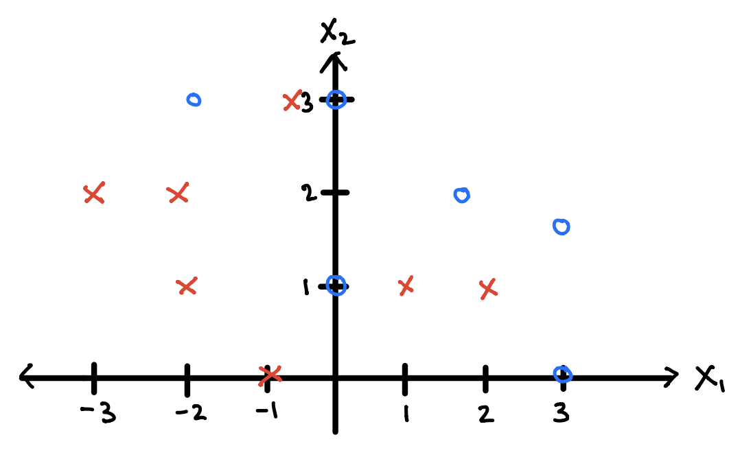
The idea. A boundary is where the classifier is equally persuaded by both classes. A confusion table then compares what is true with what you predicted. “Positive” means class 1; “false” means the prediction was wrong.
Reusable rules. The sigmoid equals at score and increases with . Here it gives the probability of class 0, so a positive score predicts 0. Always read the event inside ; the sheet’s symbol does not change the event.
counts actual 1 predicted 1; counts actual 0 predicted 0; counts missed positives; counts negatives falsely flagged positive. Each rate divides by its actual class total.
Formulas: boundary and error rates
Hint · Test the origin before counting
At the origin , the score is . That means , so this side predicts 0. Draw through and , then count each color on each side. None of the drawn points lies on the line.
Worked solution · Boundary, both confusion tables, and rates
3.1 — Set the two class probabilities equal. Because exactly when , substitute :
Draw the line through and . Above the line, , so class 0 has probability below and we predict 1. Below the line, predict 0. Use 1 at exact ties, as elsewhere in this module.
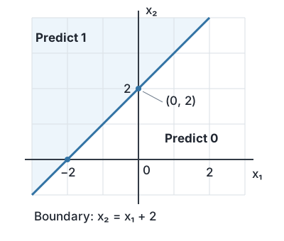
This sketch shows the decision rule. Use the original drawing above to count the observations.
3.2 — Count by true class first. Of the 7 red positives, 4 lie above the line () and 3 below it (). Of the 6 blue negatives, 2 lie above the line () and 4 below it (). The hand-drawn coordinates need not be exact to establish which side each point occupies.
| Actual class | Predict 1 | Predict 0 |
|---|---|---|
| 1 · red | TP = 4 | FN = 3 |
| 0 · blue | FP = 2 | TN = 4 |
So , . Check: points, with mistakes.
3.3 — Flip the predictions. changes each 1 to 0 and each 0 to 1. The actual labels stay fixed, so swap the two prediction columns:
| Actual class | Predict 1 | Predict 0 |
|---|---|---|
| 1 · red | TP = 3 | FN = 4 |
| 0 · blue | FP = 4 | TN = 2 |
Now , . Check: the original 8 correct predictions become 8 mistakes.
3.4 — Predict 1 for everyone. All 7 positives are found: , . All 6 negatives are falsely flagged: , . Substitute those counts into the rate formulas:
Zero missed positives does not mean a useful classifier: this one also flags every negative.
Your turn — invented extra. A classifier finds 8 of 10 actual positives and falsely flags 3 of 15 actual negatives. Find FNR and FPR.
Check your reasoning
There are missed positives, so . There are falsely flagged negatives, so . Dividing either count by all 25 observations would answer a different question.
Problem 4 · Explain the idea before calculating
Try the original questions.
- 4a. Find the Bayes classifier when .
- 4b. Explain FPR, FNR, and TPR for detecting spam.
- 4c. Give an example of correlation without direct causation. Does correlation establish causation?
- 4d. Does independence imply zero correlation? Does dependence imply nonzero correlation?
- 4e. For , with , find and the irreducible error.
- 4f. Use test mean squared error, , to choose flexibility.
- 4g. Is overfitting by a very flexible model caused by high bias?
- 4h. How do you construct a Bayes classifier? Does it minimize combined false negatives and false positives? Does it minimize false negatives alone?
The ideas and reusable rules.
Class probabilities: means the chance of label for an observation with input . Choose the largest one when errors have equal cost. For two classes, compare with .
Conditional average: hold fixed, then average the remaining randomness. For with noise independent of , noise mean , and noise variance ,
The predictable mean belongs in the prediction; only the unpredictable variation remains.
Correlation: it measures linear co-movement. For variables with finite moments,
Correlation is this covariance divided by their standard deviations, so it is zero when covariance is zero and both standard deviations are nonzero. Zero linear co-movement need not mean no relationship.
Generalization: measure error on observations not used to fit the model. With evaluation observations, actual responses , and predictions ,
At a fixed input, expected squared prediction error separates into squared bias + variance + irreducible noise. Bias is a systematic miss in the average fitted prediction. Variance is how much that prediction changes across training samples.
Formulas: class choice · error rates · averages and dependence · model flexibility
Hint · Name the population or randomness in each part
For rates, begin with “among actual spam” or “among actual non-spam.” For noise, has mean 1 and variance 2. For independence, try a symmetric and the variable . For model selection, training error and new-data error answer different questions.
Worked solution · Parts a–d
4a — Choose the more probable class. Substitute into . Since ,
Therefore predict 1 on , and 0 outside. The endpoints are ties, assigned 1 here. Check: gives probability 1; gives .
4b — Say who is in the denominator. Let positive mean spam.
| Rate | In plain words |
|---|---|
| FPR | Among actual non-spam emails, the fraction incorrectly flagged as spam |
| FNR | Among actual spam emails, the fraction incorrectly allowed through |
| TPR | Among actual spam emails, the fraction correctly caught |
Every actual spam email is either caught or missed, so . FPR is not the fraction of flagged emails that are innocent: that would use a different denominator.
4c — A common cause can move both variables. Hotter weather can increase both ice-cream sales and swimming activity. Sales and swimming can be correlated without sales causing swimming. Correlation alone does not establish causation. A shared cause, reverse causation, or other mechanisms can create the association.
4d — Independence is stronger than zero correlation. With finite variances, independence gives , so covariance is zero. Correlation is then zero if both variances are nonzero.
The reverse fails. As a counterexample, let be equally likely to be and let . These are invented values to demonstrate the claim. Since determines , the variables are dependent. But symmetry gives
Using gives . Both variances are positive, so the correlation is zero despite dependence.
Worked solution · Parts e–h
4e — Average the noise; keep its mean. Use the usual independent-noise assumption (the marginal distribution alone would not specify ). The supplied has mean 1 and variance 2. With ,
After predicting this average, the leftover error is . Its mean squared size is
Using would incorrectly count the predictable mean as unavoidable error.
4f — Compare new-data error at each flexibility. Fit each candidate using training data, calculate its on held-out observations, and select the flexibility with the lowest estimated new-data MSE. Training MSE alone can reward fitting noise.
In a practical workflow, use a validation set or cross-validation for this choice, then use a separate final test set once. Repeatedly using a “test” set to select models makes it a validation set; its minimum error is no longer an untouched final assessment.
4g — False: the issue is high variance. A very flexible model can chase accidental patterns in its training sample. On a different sample, the fitted curve may change substantially: high variance. A model too rigid to capture the pattern typically has high bias and underfits. Increasing flexibility often reduces bias while increasing variance.
4h — Choose the class with the highest conditional probability. At input , predicting class is correct with probability . Making that probability as large as possible makes the chance of error as small as possible.
With equal error costs, this minimizes expected on fresh observations. It does not guarantee the fewest realized mistakes on every finite sample; random outcomes can differ from expectations. It also need not minimize alone. Predicting 1 for everyone makes , but can create many false positives, as in Problem 3.
Your turn — invented extra. Let , with independent noise . What is the best squared-error prediction at , and what error remains unavoidable?
Check your reasoning
The conditional mean is . At , predict . The irreducible MSE is the noise variance, 9, not the standard deviation 3 and not .
Problem 5 · One order or every order?
Try the original questions. A coin lands heads with unknown probability . (a) Find the probability of exactly the sequence H, H, T. (b) In 30 flips, find the probability of 20 heads and 10 tails in any order. Assume independent flips with the same .
The idea. Multiply probabilities along one specific sequence. If several different sequences qualify, add their probabilities. Here all sequences with the same counts have equal probability, so addition becomes “number of sequences × probability of one.”
Reusable rules. Let be the number of flips and the number of heads. Then is the number of tails.
The count chooses which of the positions hold heads. The factorial is , with .
Formulas: coin sequences and counts
Hint · Does H, T, H satisfy the question?
It does not satisfy part (a), because the order differs from H, H, T. Part (b) accepts every arrangement with the requested counts, so you need a counting factor.
Worked solution · Both probabilities
5a — Multiply along the specified order. Independence lets us multiply the probabilities of H, H, and T, respectively , , and :
There is no factor of 3 because only this particular order qualifies.
5b — Count qualifying orders, then multiply. One sequence with 20 heads and 10 tails has probability . The number of distinct arrangements is
Those arrangements are mutually exclusive; only one order occurs. Add their equal probabilities:
Keep as a variable: the question asks for probability as a function of , not an estimate of the coin’s bias. As a check, if we assume , the result is .
Your turn — invented extra. A coin has . Compare the probability of H, H, T with the probability of exactly two heads in three flips.
Check your reasoning
One order: . Any order: there are qualifying sequences (HHT, HTH, THH), so .
Problem 6 · Read interactions as separate group models
Given. Let be GPA and be the supplied gender indicator: 0 for Male and 1 for Female. Salary is measured in thousands of dollars. The fitted model is:
Your tasks. (6.a) Plot both group functions for . (6.b) Find when the Male prediction is higher. (6.c) Compare full training RSS after refitting with an additional term. (6.d) Compare RSS using only Male training points. (6.e) Explain which comparisons change for test RSS. The extended model refits every coefficient:
Start with the idea. An interaction lets the effect of one predictor depend on another. Here switches on only when . Substitute the indicator before comparing the groups.
For the general model :
The group difference, Female minus Male, is . It changes with GPA when .
Adding a term expands the set of available fits. When both fits minimize unpenalized RSS on the same training data, the larger model can always set its extra coefficient to zero:
This inequality concerns training RSS. Test observations were not used to choose the coefficients.
Formula sheet: interactions and nested fits
Hint · Switch the indicator off and on
Set and then . For part 6.d, ask whether the shared-looking coefficients actually constrain the two groups to share a line. Rewrite them as one intercept and slope for each group.
Worked solution · All five parts
6.a · Plot the two regression functions
Male group. Substitute into the supplied model; both terms containing disappear:
Female group. Substitute , combine the intercept terms , and combine the slope terms :
Use these calculated points to draw the two straight lines:
| GPA | Male salary | Female salary |
|---|---|---|
| 0 | 35 | 20 |
| 1 | 40 | 30 |
| 2 | 45 | 40 |
| 3 | 50 | 50 |
| 4 | 55 | 60 |
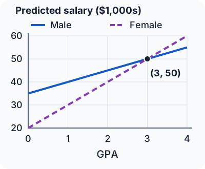
At GPA 3, both models predict $50,000. These are fitted group averages, not a causal claim about gender.
6.b · Where is the Male prediction higher?
Compare the fitted functions and by subtraction:
A higher Male prediction means a positive difference: , or . Within the requested GPA range, the answer is . The groups tie at 3; the Female prediction is higher for .
6.c · Compare total training RSS
The extended fit adds . Setting reproduces every fit available to the old model. Minimizing over this larger choice of fits therefore gives:
The new RSS is no larger. A strict decrease is not guaranteed; the extra term might provide no improvement. Although the model is quadratic in GPA for one group, it is still linear in its fitted coefficients, so ordinary least squares applies.
6.d · Compare Male training RSS
For ordinary unconstrained least squares, the Male training RSS is the same in both fits. Merely observing that for Males is not enough: the other coefficients are also refitted. The reason is that this model can fit the groups independently.
Define separate group coefficients:
Any two intercepts and slopes can be represented: choose and . Thus the original fit independently minimizes a Male line’s RSS and a Female line’s RSS. The extended fit independently minimizes a Male line’s RSS and a Female quadratic’s RSS.
The Male task is identical in both cases: minimize . Its optimal training RSS cannot change. With at least two distinct Male GPA values, its fitted intercept and slope are also identical. This conclusion assumes unpenalized least squares with no constraints linking the group coefficients.
6.e · What changes on test data?
All groups combined: there is no guaranteed ordering of test RSS. The Female quadratic may capture useful curvature or fit training noise, so total test RSS may fall, rise, or stay equal.
Male points only: the two fits make the same Male predictions at every GPA when the Male line is identifiable (at least two distinct training GPA values). On the same Male test points, their test RSS is therefore equal too. Without an identifiable Male line, off-training predictions need not be unique, even though minimum Male training RSS is equal.
Invented transfer check. Change only the supplied interaction coefficient from 5 to 3, making the prediction . Do the two group lines cross in the GPA range ?
Check your reasoning
Setting gives Male salary ; setting gives Female salary . Their difference is . Setting it to zero gives , outside . The Male prediction is higher throughout the requested range. At GPA 4, the predictions are and , in thousands of dollars.
Problem 7 · Separate the fitted intercept from the noise mean
Given. The model is , initially with and . The five supplied observations are:
| −2 | −3.5 |
| −1 | −3 |
| 0 | 0 |
| 1 | 3 |
| 2 | 3.5 |
Your tasks. (7.a) Fit the intercept and slope. (7.b) Find 95% confidence intervals as functions of . (7.c) Find when to reject . (7.d) Explain what changes if the noise instead has distribution . Keep the printed dataset fixed in part 7.d.
Start with the idea. The fitted line estimates the average response. If the noise has a nonzero average , that average shifts the line’s intercept:
Here is assumed constant. Calling the mean-response intercept , an ordinary fitted intercept estimates . To estimate the model’s original intercept, subtract the known noise mean:
For fitting, define and . Then:
For independent Gaussian errors with supplied standard deviation , fixed observed values, and observations:
A 95% interval is estimate . Subtracting a known constant shifts the intercept interval without changing its width.
Formula sheet: fitting a line · coefficient uncertainty · hypothesis tests · noise with a nonzero mean
Hint · Use symmetry, then identify what the intercept estimates
Both coordinate means are zero. This makes the fitted mean-response intercept zero and removes the term from its variance. In part 7.d, distinguish the fitted mean-response line from the structural parameter in the model statement.
Worked solution · All four parts
7.a · Fit the coefficients
Means. The five values sum to 0, and the five values sum to 0. With , and .
Spread. With , square the supplied values:
Joint variation. Because both means are zero, multiply each supplied pair and add:
Slope and intercept. Substitute , , , and :
The fitted line is . Here the original noise mean is zero, so the fitted intercept estimates directly.
7.b · Find the confidence intervals
Slope. The supplied noise standard deviation is , and , so . With fitted slope 2:
or approximately .
Intercept. Use , , , and noise standard deviation :
With fitted intercept 0, its interval is:
or approximately . These use the supplied noise variance, so the normal multiplier is 1.96.
7.c · When do we reject a zero slope?
The fitted slope 2 is a distance from the null slope 0. Reject at the two-sided 5% level when this exceeds the half-width :
Solving for positive gives:
At larger noise levels, zero falls inside the slope’s interval. A value exactly at the endpoint is retained under our strict rejection rule.
7.d · What if the noise mean is 1?
The fitted mean-response line stays the same. For the same printed observations, ordinary least squares still returns intercept and slope . Changing an assumption does not change the data’s least-squares line.
The original intercept’s interpretation changes. With the supplied new noise mean :
The fitted intercept 0 now estimates . Subtract the known mean to estimate :
The variance is still . Therefore the 95% interval for the original intercept shifts down by 1 and keeps its half-width:
The slope estimate remains 2, its interval remains , and the rejection condition remains (approximately). The predicted average response is still .
Invented transfer check. Keep the printed data, but suppose the known noise mean is −2 and its standard deviation is . Find the estimate and 95% interval for the original intercept .
Check your reasoning
The data still give mean-response intercept . Subtracting the known noise mean gives . With , , and , its standard error is . The interval is , approximately . Its center changes; its uncertainty comes from the variance, which has not changed.
Problem 8 · Why random guessing gives a diagonal ROC
Try the original questions. A classifier ignores the input and flips an independent coin: predict 1 with probability and 0 otherwise. (a) Prove its ROC is a straight line as varies. (b) Find the AUC. (c) Without information about the input or true label, can you systematically achieve a higher or lower AUC?
The idea. An ROC curve plots the fraction of negatives you flag against the fraction of positives you catch. A useful signal lets you catch positives more often than you flag negatives. An independent coin treats both groups identically.
Reusable rules. The horizontal coordinate is the false-positive rate; the vertical coordinate is the true-positive rate. is the predicted label, and is the actual label.
Vary a threshold or classifier parameter to trace the curve. AUC is the area under that curve in the unit square. One fixed value of gives a single operating point, not a whole curve.
Hint · What changes when you learn the true class?
Nothing changes the coin. Whether the observation is actually positive or negative, the probability of predicting 1 is still .
Worked solution · The diagonal and its area
8a — Calculate each coordinate. The coin is independent of the actual label. Among actual negatives it predicts 1 with probability , so . Among actual positives it also predicts 1 with probability , so .
Thus the curve is , a diagonal from to . For example, gives ; gives .
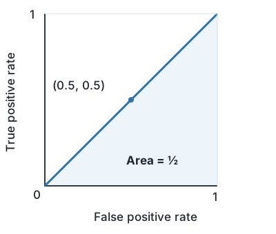
8b — Find the area of the triangle. The area below that diagonal has base 1 and height 1:
8c — No information means no systematic ranking advantage or disadvantage. If a score or prediction is independent of the true label, positives and negatives have the same score distribution. Every threshold therefore produces equal TPR and FPR. You cannot systematically achieve a population AUC above or below without information related to the label. Flipping an independent coin’s outputs still gives an independent coin.
A measured AUC on a finite random sample can be above or below by chance. Also, knowing that one class is more common can help accuracy through majority guessing, but supplies no way to rank individual positives ahead of negatives; it does not improve AUC.
Your turn — invented extra. An independent random classifier flags 30% of observations. What are FPR, TPR, and FNR? Would raising that rate to 80% improve its population AUC?
Check your reasoning
With , FPR and TPR are both 0.3, and FNR is . Raising to 0.8 moves along the same diagonal. The family still has AUC .
Practice
Close the worked solutions and choose the method yourself. The questions below are invented extra exercises, not additional questions from the PDF. Try a full round, then use the feedback to decide which original problem to redo.
Can you do it without the page?
Before calling a problem learned, check that you can do all four:
- Recognize: identify the response, probability event, or error population before choosing a formula.
- Calculate: show the rule, substitute named values, and check the result’s sign, range, and units.
- Explain: say why that rule fits, and name one tempting wrong approach.
- Transfer: solve a changed version and repeat the original after a delay without notes.
For a final rehearsal, open the original sheet, keep these solutions closed, and work through all eight problems. For each miss, write one sentence: “I used ___; I should use ___ because ___.” Then redo that problem from a blank page.