Module 4 · Categories, interactions, and curves

One picture: a prediction is a starting value plus a few contributions. This module changes what those contributions can be: a group adjustment, a changing slope, or a curve.

Slides → small steps → practice. Browse the original slides above each topic, or click to enlarge. Keep the formula sheet nearby.

1. The same machine, different inputs

Coefficient = multiplier

In Module 3, the model was

$$Y=\beta_0+\beta_1X+\varepsilon.$$

$Y$ is the outcome; $X$ is an input. The intercept $\beta_0$ is the starting value. The coefficient $\beta_1$ multiplies the input. Noise $\varepsilon$ is the variation the rule does not explain.

Hat = estimate from data

The true coefficients are unknown. We fit estimates, marked with hats, and predict without adding unknown noise:

$$\widehat Y=\widehat\beta_0+\widehat\beta_1X.$$

With $p$ input columns, add their contributions:

$$\widehat Y=\widehat\beta_0+ \sum_{j=1}^{p}\widehat\beta_jX_j.$$

$j$ selects a column; $p$ excludes the intercept. A column can contain a switch, a product, or a square. Least squares still chooses the weights that minimize total squared prediction error.

2. Two categories: use a switch

Original slides · Categorical InputsOpen PDF ↗

Slide 4 of 6

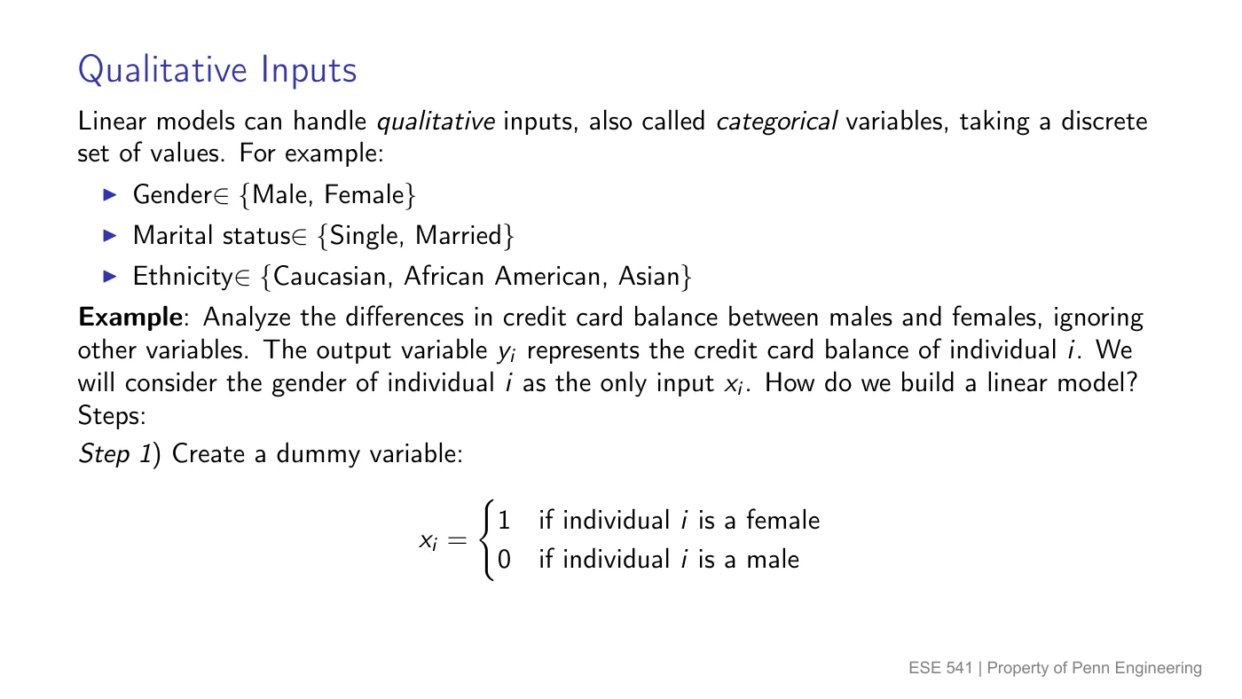
0 means off; 1 means on

A dummy variable, or indicator, switches a group adjustment on or off. Let $D=1$ for a student and $D=0$ for a nonstudent:

$$D=\begin{cases} 1 & \text{student},\\ 0 & \text{nonstudent}. \end{cases}$$

The rule is starting value + adjustment × switch:

$$\widehat Y=\widehat\beta_0+\widehat\beta_1D.$$

Substitute the switch before interpreting

Group	Substitute	Prediction
Nonstudent	$D=0$	$\widehat\beta_0$
Student	$D=1$	$\widehat\beta_0+\widehat\beta_1$

The group coded 0 is the reference or baseline. $\widehat\beta_0$ predicts that group; $\widehat\beta_1$ is the student-minus-nonstudent difference.

Invented example: $\widehat Y=40+15D$ dollars. Nonstudents get $40+15(0)=40$; students get $40+15(1)=55$.

With only this switch and an intercept, least squares predicts each group’s sample average. With other inputs included, compare groups at the same values of those inputs.

Try it — invented: in $\widehat Y=60-8D$, $D=1$ means premium membership. Predict for both groups. Rule: binary categories.

Show the answer

Regular: $D=0$, so $60-8(0)=60$. Premium: $D=1$, so $60-8(1)=52$. A negative adjustment lowers the prediction by 8.

3. Several categories: one baseline, the rest switches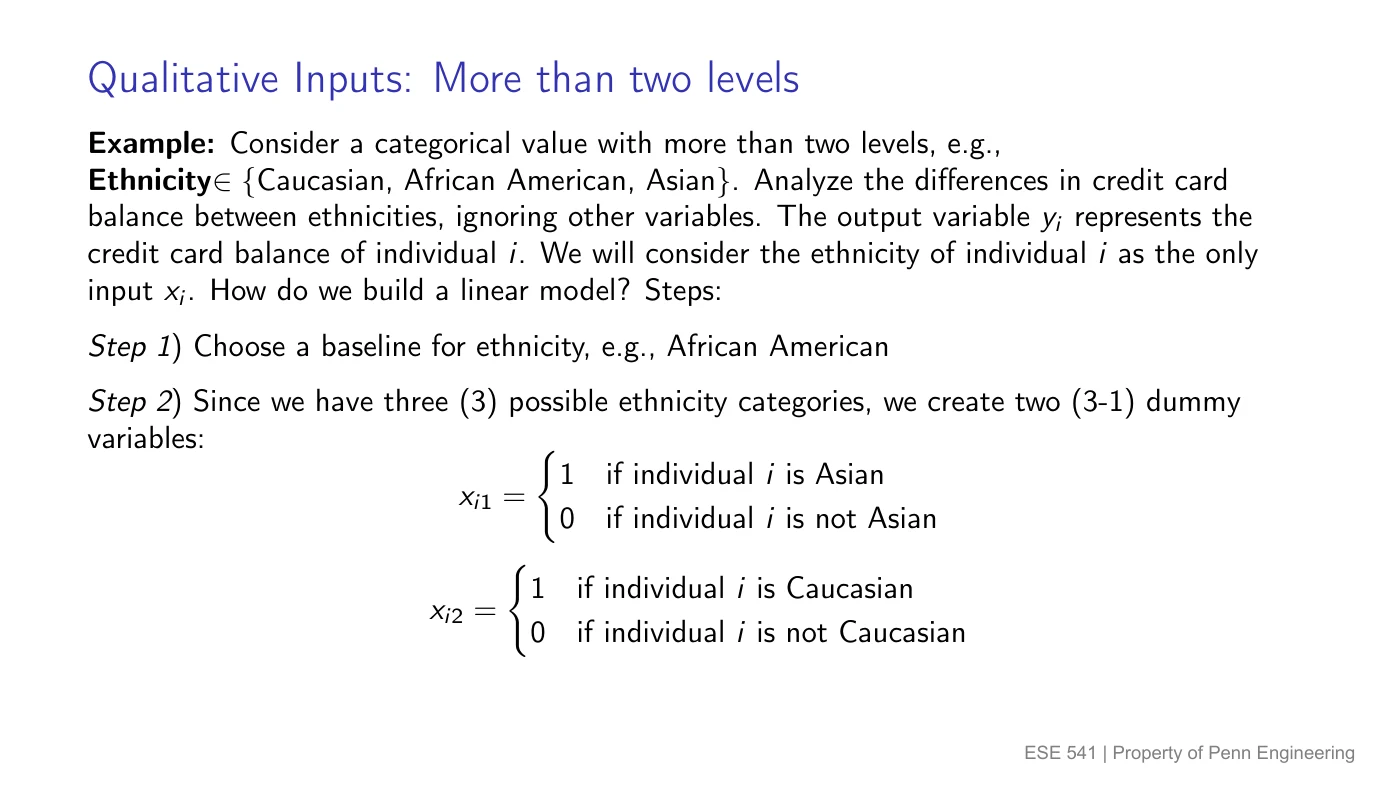

Original slides · More Categorical InputsOpen PDF ↗

Slide 2 of 4

One group supplies the starting value

For Basic, Plus, and Pro plans, choose Basic as the reference. Define $D_\text{Plus}=1$ for Plus and $D_\text{Pro}=1$ for Pro; otherwise each is 0.

$$\begin{aligned} \widehat Y&=\widehat\beta_0 +\widehat\beta_P D_\text{Plus}\\ &\quad +\widehat\beta_R D_\text{Pro}. \end{aligned}$$

$\widehat\beta_P$ and $\widehat\beta_R$ are fitted adjustments for Plus and Pro.

Plan	Plus switch	Pro switch	Prediction
Basic	0	0	$\widehat\beta_0$
Plus	1	0	$\widehat\beta_0+\widehat\beta_P$
Pro	0	1	$\widehat\beta_0+\widehat\beta_R$

Remember K − 1

$K$ categories need $K-1$ switches when there is an intercept. All switches are off for the reference. Coding the groups $1,2,3$ instead would impose equally spaced predictions.

Invented coefficients: baseline 20, Plus adjustment 5, Pro adjustment $-3$. Predictions are $20$, $20+5=25$, and $20-3=17$. Plus exceeds Pro by $5-(-3)=8$.

Changing the reference changes the coefficient meanings, but preserves the fitted predictions.

Why leave one switch out?

Exactly one of all $K$ group switches is on in each row. They therefore add to 1, duplicating the intercept column of ones. Leaving one out lets the model separate the weights.

4. Interactions: one input changes another’s effect

Original slides · Interaction TermsOpen PDF ↗

Slide 2 of 7

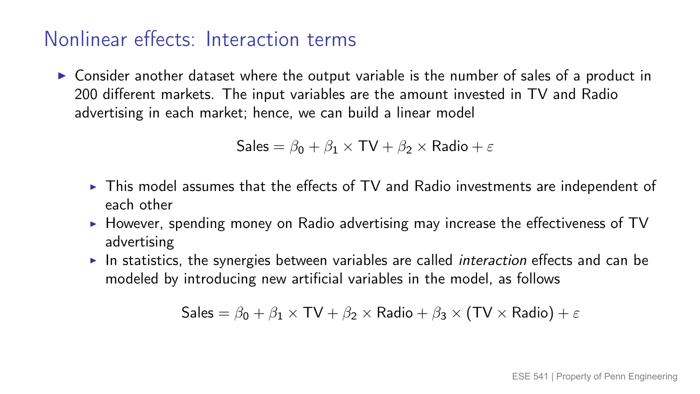
Multiply two inputs to make a new column

Let $T$ be TV spending, $R$ radio spending, and $\widehat S$ predicted sales. An additive model gives each input a fixed slope:

$$\widehat S=\widehat\beta_0+ \widehat\beta_1T+\widehat\beta_2R.$$

An interaction lets one input change the other’s slope. Literally calculate a new feature, $TR=T\times R$, and give it a coefficient:

$$\begin{aligned} \widehat S&=\widehat\beta_0+ \widehat\beta_1T+\widehat\beta_2R\\ &\quad +\widehat\beta_3TR. \end{aligned}$$

Read the fitted multipliers

These numbers come from slide 3 of the interaction deck. Each coefficient is a fitted multiplier; the intercept is the baseline.

Term	Coefficient	Std. Error	t
Intercept	6.7502	0.248	27.23
TV	0.0191	0.002	12.70
Radio	0.0289	0.009	3.24
TV × Radio	0.0011	0.000	20.73

Calculate each contribution, then add

Invented inputs: take $T=100$, $R=20$ in the model’s input units. Use the slide’s fitted coefficients above. The new product is $TR=100(20)=2000$.

• Intercept: start at $6.7502$.
• TV contribution: $0.0191(100)=1.91$.
• Radio contribution: $0.0289(20)=0.578$.
• Product contribution: $0.0011(2000)=2.2$.

Prediction = sum of the four contributions:

$$\begin{aligned} \widehat S&=6.7502+1.91+0.578+2.2\\ &=11.4382. \end{aligned}$$

Group the TV terms to find its slope

Hold $R$ fixed. Everything multiplying $T$ becomes its slope:

$$\begin{aligned} \widehat S&=(\widehat\beta_0+\widehat\beta_2R)\\ &\quad +(\widehat\beta_1+\widehat\beta_3R)T. \end{aligned}$$ $$\text{TV slope}=\widehat\beta_1+\widehat\beta_3R.$$

Using the slide’s $\widehat\beta_1=0.0191$, $\widehat\beta_3=0.0011$ and our assumed $R=20$:

$$\text{TV slope}=0.0191+0.0011(20)=0.0411.$$

One extra TV unit now adds 0.0411 predicted sales units. The coefficient 0.0191 is TV’s slope only when radio spending is 0.

Similarly, radio’s slope is $\widehat\beta_2+\widehat\beta_3T$. A positive interaction makes either slope increase with the other input; a negative interaction decreases it.

Hierarchy principle: keep $T$ and $R$ when including $TR$, even if their individual tests are not significant. Keep the starting effects when modeling how they change.

Standard error = how much the estimate might bounce

Collect another sample, refit, and the coefficient will change. Std. Error, or SE, estimates the size of that sample-to-sample variation.

t = effect divided by uncertainty

To test the true interaction coefficient $\beta_3=0$, ask: how many standard errors is the estimate from zero?

$$t=\frac{\widehat\beta_3-0} {\operatorname{SE}(\widehat\beta_3)}.$$

Use the module’s approximate two-sided rule: reject zero when $|t|>2$; otherwise fail to reject, including at $|t|=2$.

Here $|20.73|>2$: strong evidence of a nonzero interaction under the model’s assumptions. Statistical evidence alone proves neither causation nor improved predictions on new data.

Read rounded tables carefully. SE printed as 0.000 means a tiny positive value rounded down. It does not mean zero uncertainty. The printed values cannot reproduce the exact t-statistics.

How small is that interaction SE?

Rearrange $t=\widehat\beta_3/\operatorname{SE}$ to get $\operatorname{SE}=\widehat\beta_3/t$. Using the rounded coefficient 0.0011 and reported $t=20.73$ gives approximately $0.0011/20.73=0.0000531$. This is an approximate reconstruction, not the original unrounded SE.

5. Category interactions: let groups have different slopes

Original slides · Interaction TermsOpen PDF ↗

Slide 6 of 7

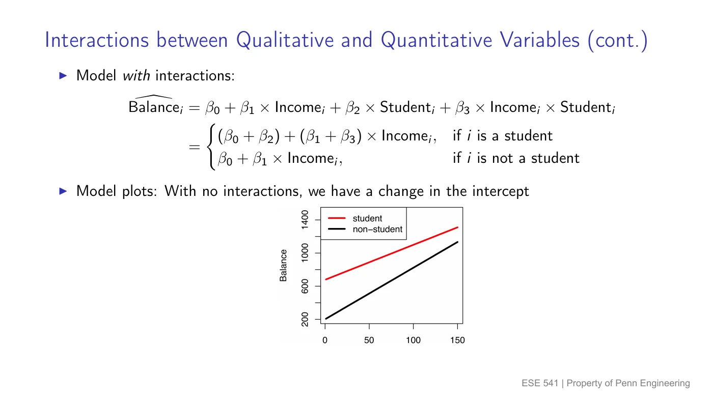
First switch on a different starting value

Let $X$ be income, $D=1$ for students and $D=0$ for nonstudents. For predicted balance $\widehat B$:

$$\widehat B=\widehat\beta_0+ \widehat\beta_1X+\widehat\beta_2D.$$

$\widehat\beta_2$ shifts the student starting value. Both groups still have slope $\widehat\beta_1$: parallel lines.

Then switch on an extra slope

Add $XD$: it equals 0 for nonstudents and $X$ for students.

$$\begin{aligned} \widehat B&=\widehat\beta_0+ \widehat\beta_1X+\widehat\beta_2D\\ &\quad +\widehat\beta_3XD. \end{aligned}$$

Substitute first; read second:

$$\begin{aligned} D=0:\quad\widehat B &=\widehat\beta_0+\widehat\beta_1X,\\ D=1:\quad\widehat B &=(\widehat\beta_0+\widehat\beta_2)\\ &\quad +(\widehat\beta_1+\widehat\beta_3)X. \end{aligned}$$

$\widehat\beta_2$ changes the intercept; $\widehat\beta_3$ changes the slope. At income $X$, the student-minus-nonstudent gap is $\widehat\beta_2+\widehat\beta_3X$.

Try it — invented: $\widehat B=20+2X+10D+3XD$, with balance in dollars and income in thousands of dollars. Find both lines, then predict at $X=4$. Rule: category interactions.

Show the answer

• $D=0$: $\widehat B=20+2X$. At $X=4$, $20+2(4)=28$ dollars.
• $D=1$: $\widehat B=(20+10)+(2+3)X=30+5X$. At $X=4$, $30+5(4)=50$ dollars.

The gap rule gives $10+3(4)=22$, matching $50-28$. For parallel lines, the interaction coefficient would have to be 0.

For $K$ groups, multiply each of the $K-1$ switches by $X$ to allow a separate slope per group.

6. Curves are still possible in linear regression

Original slides · Nonlinear EffectsOpen PDF ↗

Slide 2 of 4

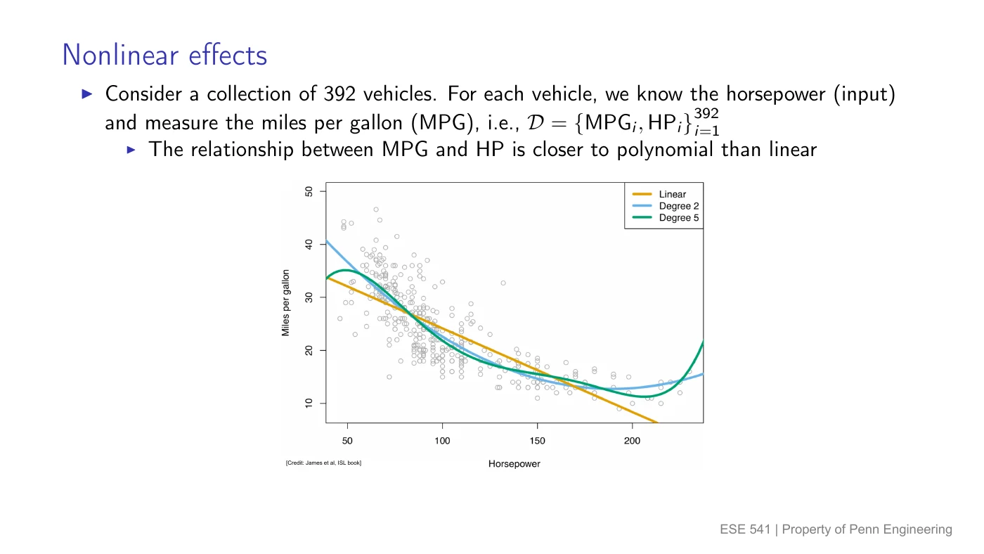
A curve starts with calculated columns

To model curvature, such as fuel efficiency changing with horsepower, add $X^2$ as a column:

$$\widehat Y=\widehat\beta_0+ \widehat\beta_1X+\widehat\beta_2X^2.$$

This is quadratic. A cubic adds $\widehat\beta_3X^3$; degree $k$ means powers through $X^k$.

Linear in the weights

The inputs are squared or cubed. The fitted weights still multiply known columns and add, so this remains linear regression.

Invented example: at $X=2$, the columns $[1,X,X^2]$ become $[1,2,4]$. With weights $1,3,2$:

$$\widehat Y=1+3(2)+2(4)=15.$$

Remember: calculate columns first; fit weights second. Extra terms can follow a real curve or random training bumps. Check new data to tell whether they help.

7. Shared practice Q4: straight line versus cubic

View the original practice sheet (includes solutions)

Original practice sheet · Module 3 and 4 Practice Problems - SolutionsOpen PDF ↗

Slide 2 of 3

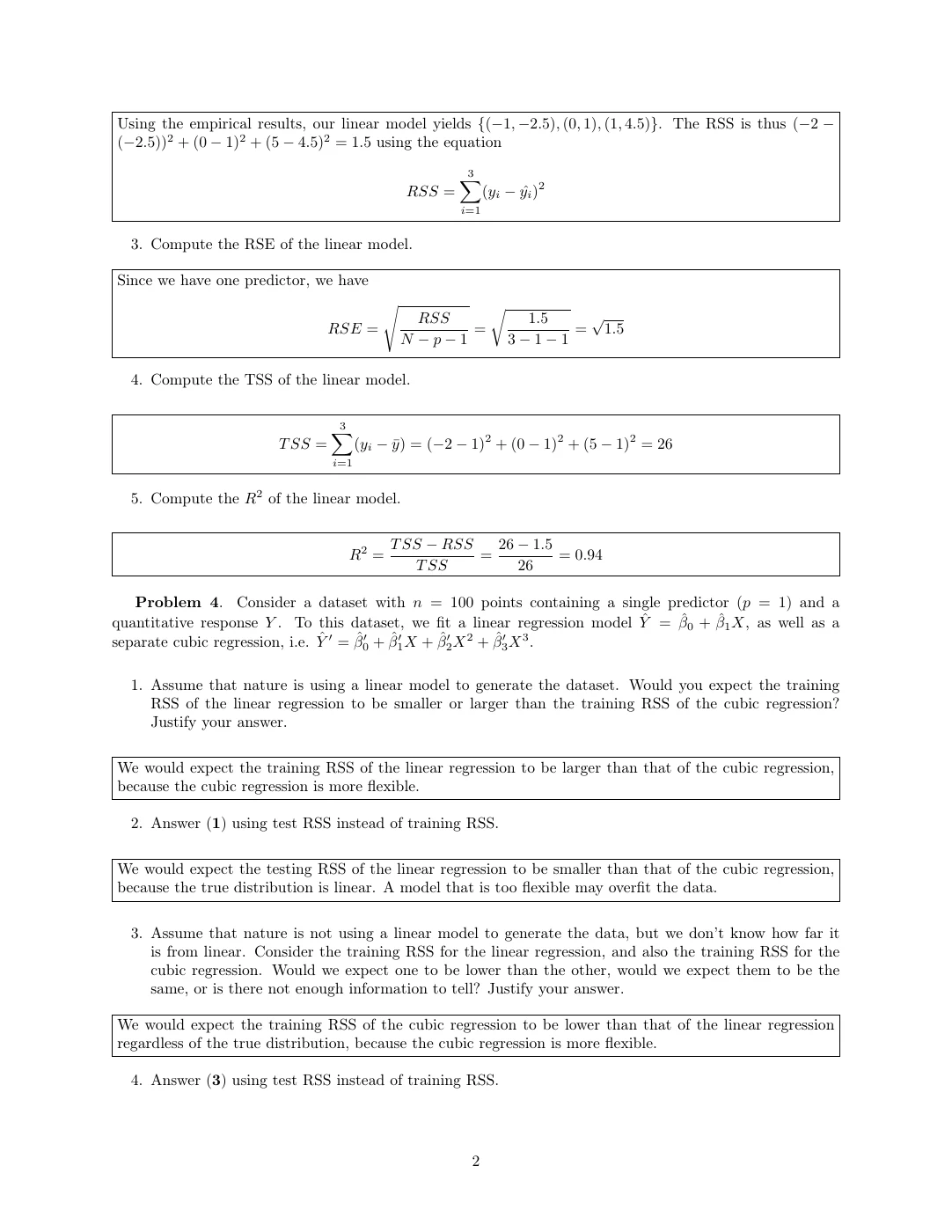
Given: 100 observations, one original input $X$, and numerical outcome $Y$. Fit both models by ordinary least squares on the same training data:

$$\begin{aligned} \widehat Y_\text{linear}&=a_0+a_1X,\\ \widehat Y_\text{cubic}&=c_0+c_1X\\ &\quad+c_2X^2+c_3X^3. \end{aligned}$$

$a$ and $c$ are separate fitted coefficients. RSS is the total squared miss: $\mathrm{RSS}=\sum_i(y_i-\widehat y_i)^2$, using actual output $y_i$ and prediction $\widehat y_i$ for observation $i$.

Circle TRAIN or TEST first: training data chooses the weights; test data checks them without refitting.

1. Linear truth: which has smaller training RSS?
2. Linear truth: which do you expect to have smaller test RSS?
3. Nonlinear truth: which has smaller training RSS?
4. Nonlinear truth, amount unknown: which has smaller test RSS?

Rules: polynomial features and training versus test RSS.

The move to remember: switch off the extra terms

Set $c_2=c_3=0$, then $c_0=a_0$ and $c_1=a_1$. The cubic now copies the line exactly. Its best training fit therefore cannot be worse:

$$\mathrm{RSS}_\text{cubic, train} \leq\mathrm{RSS}_\text{linear, train}.$$

Answer all four cases

1. Linear truth, training: cubic RSS is smaller or equal. It can copy the line and improve on it if extra terms help. Equality is possible.

2. Linear truth, test: expect the line to do better. It has the right shape already; extra terms may learn training noise. This expectation is not a guarantee for every dataset.

3. Nonlinear truth, training: cubic RSS is again smaller or equal. The ability to copy the line does not depend on what generated the data.

4. Nonlinear truth, test: not enough information. Extra terms might capture useful curvature or mostly noise. Compare on the same held-out observations, without refitting.

The cubic has $p=3$ input columns, $X,X^2,X^3$, and four coefficients including its intercept.

8. Shared practice Q6: fit a quadratic by renaming a column

View the original practice sheet (includes solutions)

Original practice sheet · Module 3 and 4 Practice Problems - SolutionsOpen PDF ↗

Slide 3 of 3

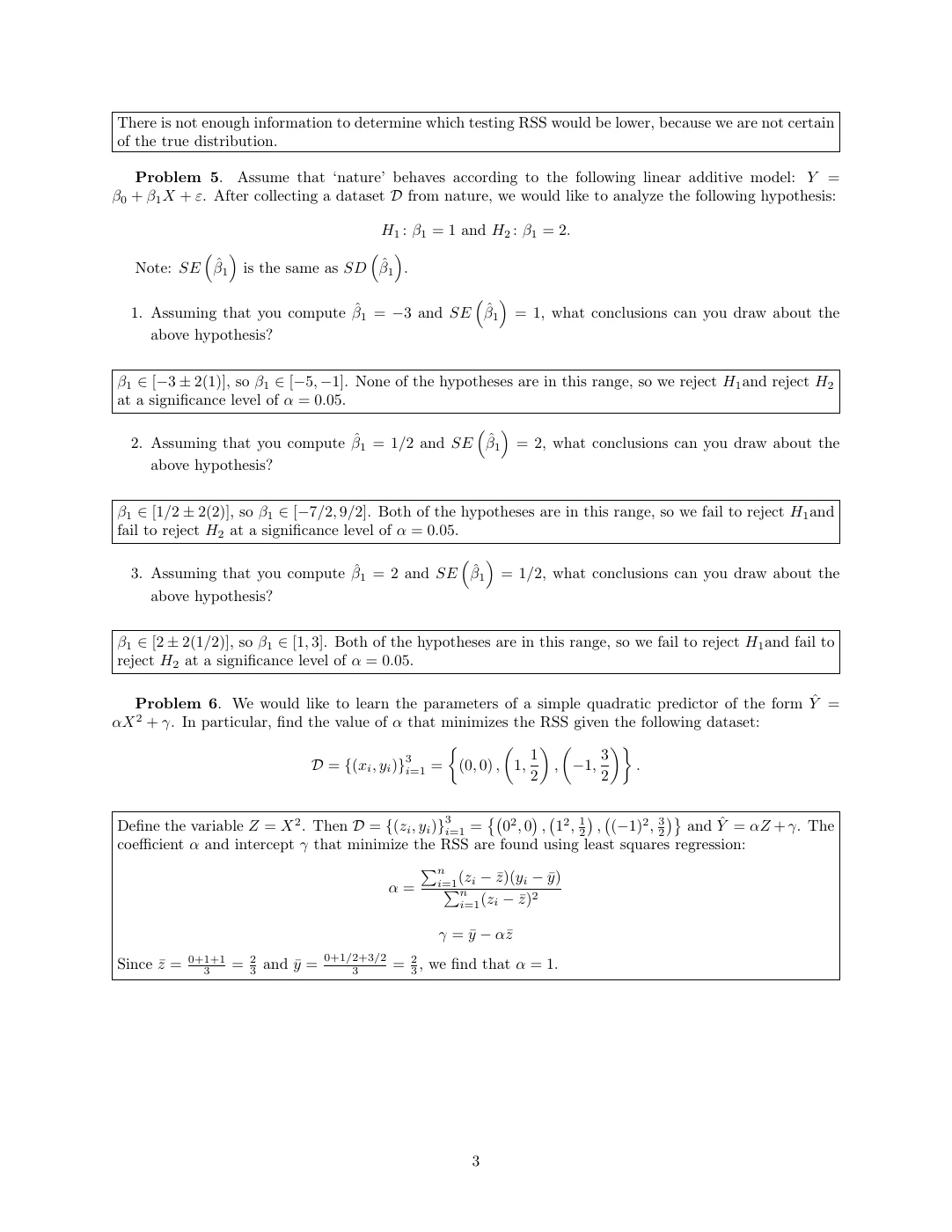
Given: fit $\widehat Y=\alpha X^2+\gamma$ to $(0,0)$, $(1,1/2)$, and $(-1,3/2)$. Find $\alpha$ minimizing RSS. Here $\alpha$ weights $X^2$, and $\gamma$ is the fitted intercept. Count $p=1$ input column, $X^2$; there is no $X$ term.

Rules: transformed least squares and RSS.

Same squared input → same prediction

Set $z_i=x_i^2$, where $i$ selects an observation. The model becomes a line, $\widehat y_i=\alpha z_i+\gamma$:

Supplied $x_i$	Supplied $y_i$	Calculated $z_i$
$0$	$0$	$0$
$1$	$1/2$	$1$
$-1$	$3/2$	$1$

Squaring makes $1$ and $-1$ identical inputs. Squared error favors their average output as their shared prediction.

Fast solution: two input values, two group averages

At $z=0$: the only output is 0. Since $\widehat y=\alpha(0)+\gamma=\gamma$, choose $\boxed{\gamma=0}$.

At $z=1$: the average output is $(1/2+3/2)/2=1$. Since $\widehat y=\alpha(1)+0$, choose $\boxed{\alpha=1}$.

Thus $\widehat Y=X^2$. This line hits both group averages, so it minimizes the total squared error.

Check RSS. At original inputs $0,1,-1$, predictions are $0,1,1$. Subtract predictions from the supplied outputs $0,1/2,3/2$:

$$\begin{aligned} \mathrm{RSS}&=(0-0)^2+(\tfrac12-1)^2\\ &\quad +(\tfrac32-1)^2\\ &=0+\tfrac14+\tfrac14=\tfrac12. \end{aligned}$$

The two outputs at $z=1$ differ, so one shared prediction cannot hit both.

The general rule when that shortcut is unavailable

For $n$ observations, calculate averages $\bar z=\sum_i z_i/n$ and $\bar y=\sum_i y_i/n$. Then use the usual straight-line rules:

$$\alpha=\frac{S_{zy}}{S_{zz}}, \qquad \gamma=\bar y-\alpha\bar z.$$

The numerator measures how the columns move together; the denominator measures input spread:

$$S_{zy}=\sum_i(z_i-\bar z)(y_i-\bar y),$$ $$S_{zz}=\sum_i(z_i-\bar z)^2>0.$$

Verify Q6 with the general calculation

Means: $n=3$, new inputs $0,1,1$, and supplied outputs $0,1/2,3/2$ give

$$\bar z=\frac{0+1+1}{3}=\frac23, \qquad \bar y=\frac{0+\tfrac12+\tfrac32}{3}=\frac23.$$

Center: subtract $2/3$ from each column:

Row	$z_i-\bar z$	$y_i-\bar y$
1	$-2/3$	$-2/3$
2	$1/3$	$-1/6$
3	$1/3$	$5/6$

Multiply and add for $S_{zy}$:

$$\begin{aligned} S_{zy}&=(-\tfrac23)(-\tfrac23)\\ &\quad +(\tfrac13)(-\tfrac16)\\ &\quad +(\tfrac13)(\tfrac56)\\ &=\tfrac49-\tfrac1{18}+\tfrac5{18}=\tfrac23. \end{aligned}$$

Square and add for $S_{zz}$:

$$\begin{aligned} S_{zz}&=(-\tfrac23)^2+(\tfrac13)^2+(\tfrac13)^2\\ &=\tfrac49+\tfrac19+\tfrac19=\tfrac23. \end{aligned}$$

Divide to find the slope: $\alpha=(2/3)/(2/3)=1$.

Find the intercept: $\gamma=\bar y-\alpha\bar z=2/3-1(2/3)=0$. Both answers match the shortcut.

9. The five questions to ask

• Group label? Switch its adjustment on or off.
• $K$ groups? One reference, $K-1$ switches.
• Product term? Group terms to read the changing slope.
• Power of an input? Calculate the column, then fit its weight.
• More flexible model? Training can improve; test performance must be checked.

Open the formula sheet to reuse the rules with different numbers.