DeepSeek-V4.1-Flash: doing less repeated work

Suppose a model must answer a question about a long book. It needs useful information from the book, but repeatedly preparing and reading all of that information is expensive.

This paper combines several ways to reduce that repeated work. To understand its diagram, follow two questions: what information is kept, and what calculation still happens?

Read along: the official technical report, beginning with Figure 3. The small numbers below are teaching examples.

Start with the job

Given “The key is in the blue box. The box is…”, the model scores possible next pieces of text. Each piece, or token, begins as a row of numbers. Layers update those rows; the final row helps score the next token.

Attention lets a row mix information from earlier positions. A small network then transforms the row. If that operation is unfamiliar, work through one attention calculation first.

The changing rows are hidden states. The stored rules that transform them are weights. Processing a prompt changes the states; ordinary inference keeps the weights fixed.

Why change attention?

Imagine there are 16 earlier positions to read. There are several different ways to make reading cheaper:

Try this	The paper’s term	What becomes limited
Keep only nearby positions	Sliding-window attention, SWA	Direct access to distant information in that branch
Pack pairs into 8 entries	Compression	How much original detail can be recovered
Read 2 chosen entries	Sparse attention	Direct access to unselected entries
Prepare entries once for several layers	KV reuse	Independent preparation at every layer

Compression reduces what is stored. Selection reduces what is read. These can be combined: store 8 packed entries, then read 2. The counts alone do not tell us how much faster the entire model will be.

Now read §2.3: Compressed Sparse Attention 2, abbreviated CSA2. It combines a local window with selected global entries. In CSA2(2, …), the 2 means global positions are packed at a two-to-one ratio. A 1 means that packing is absent.

Same information, a fresh question

Attention uses keys to calculate relevance and values as the information to mix. Keeping those prepared arrays gives us a KV cache. A layer’s current query determines how it reads them.

Suppose two stored values are 10 and 30:

• One query gives them shares of 80% and 20%: the result is 14.
• Another gives them shares of 10% and 90%: the result is 28.

The values stayed the same. The way they were combined changed. That is why reusing stored information can still produce a new result.

Now read Figure 4 in §2.3.1. Its three labels describe which preparation steps happen:

Label	Prepared global information	Selected locations
Full	Make it	Choose them
Reuse	Keep it	Keep the previous selection
Reindex	Keep it	Choose again

Every mode still computes a new main query, local-window keys and values, and attention output. Full names the preparation mode; its global attention still reads a selected subset.

Read the two halves of Figure 3

Read each stack from bottom to top. Focus first on the two large boxes and the line carrying encoder hidden states to the decoder.

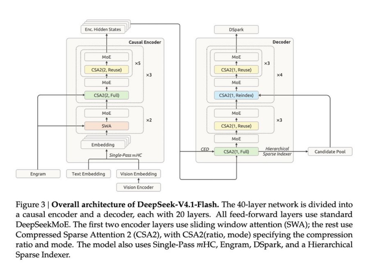
The causal encoder has 20 layers. It prepares states using only information available up to each position. The decoder has another 20 layers. It prepares its global KV from the encoder’s final states, then shares that memory across decoder layers.

Images enter through a separate network, the vision encoder, that converts them into features for the language model.

This separation saves repeated preparation of a long prompt. Each newly generated position still passes through both halves. Read §2.2, Causal Encoder-Decoder.

Each attention–MoE pair counts as one layer. A dotted ×5 repeats the drawn structure five times; it does not establish that those layers have identical weights.

Give the remaining boxes a job

MoE: choose which networks run. Remember the network that transforms a row? A mixture of experts offers several alternatives and a router selects a few. This model runs one shared expert plus six selected from 384 routed experts per layer. The skipped networks still occupy storage. §4.2.1.

Engram: look up a local pattern. Nearby token IDs address learned tables; the retrieved numbers contribute to the current state. These tables are learned model memory. §2.4.2.

mHC: carry several state paths. An ordinary residual path preserves a row and adds an update to it. mHC keeps several streams and mixes them. Single-Pass mHC arranges that mixing to reduce memory movement. §2.4.1.

Hierarchical indexer: narrow the search. An initial broad search keeps a candidate pool. Later selections search within that pool. A useful entry left outside the pool cannot be chosen through that restricted search. §2.3.2.

DSpark: draft, then verify. A small model proposes several tokens. The main model checks the continuation before accepting it. Useful drafts can reduce sequential waiting. §2.4.3.

Is this recurrence?

Sharing prepared data and sharing an update rule are different choices. CSA2’s Reuse label concerns prepared data. Shared-depth recurrence applies the same learned block again to an evolving state. Work through that distinction.

Check the idea

A Reuse layer reads the same values at the same locations. Why can its output change?

Its fresh query can give those values different shares—just as our two mixtures of 10 and 30 produced 14 and 28. It also computes fresh local attention and a new network update.

What would show that these shortcuts are worthwhile?

Measure answer quality alongside processing time and memory at comparable budgets. Then look for an ablation: remove one component and see what changes. The architecture describes possible savings; the experiments test whether the resulting tradeoff is useful. This lesson does not independently reproduce the report’s benchmarks.

How other models fit this map

Compare published designs and what remains unknown

Sources checked September 10, 2026. These describe particular models and variants.

Model	Connection to the ideas above
Qwen3.8-Flash-Next	Three Gated DeltaNet layers per sparse-attention layer combine recurrence across tokens with selected context reading. Updating a state as tokens arrive is different from repeating a block across depth. §2.1
Gemma 4	Local/global attention and cross-layer KV sharing in the E2B/E4B variants reuse prepared data. Sharing an entire update rule is a separate property. §2
OpenAI’s deployed models	The cited Parameter Golf discussion and An Alien Mind essay do not specify a deployed model’s complete architecture. Read what those comments establish.

A long pause or a long written explanation cannot identify which internal mechanism a model uses.

Reference

Count the layers and inspect the implementation details

Part	Count
Encoder: 2 local layers + 3 groups of (1 Full + 5 Reuse)	20
Decoder: (1 Full + 3 Reuse) + 4 groups of (1 Reindex + 3 Reuse)	20
Backbone total	40

The vision encoder and speculative drafter are additional components. Engram enters encoder layers 2 and 15 when numbering starts at 1; the report numbers them 1 and 14 from zero.

The candidate pool holds at most 16,384 positions; each final global selection contains up to 512 entries. The first broad scan still costs work.

The initial processing of a prompt is prefill. For decoder local attention, this implementation replays the last 128 prompt tokens. That bounded replay approximates the full local dependency history. Generating new tokens is decode; each new position still traverses both halves. See §§2.2 and 3.2.2 of the report.

Inspect the original layer map or try the smaller attention, routing, and recurrence calculations.